| Date | May 2022 | Marks available | 1 | Reference code | 22M.3.AHL.TZ2.2 |
| Level | Additional Higher Level | Paper | Paper 3 | Time zone | Time zone 2 |
| Command term | State | Question number | 2 | Adapted from | N/A |
Question
This question compares possible designs for a new computer network between multiple school buildings, and whether they meet specific requirements.
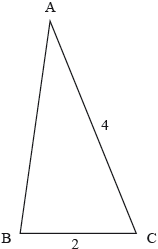
A school’s administration team decides to install new fibre-optic internet cables underground. The school has eight buildings that need to be connected by these cables. A map of the school is shown below, with the internet access point of each building labelled .

Jonas is planning where to install the underground cables. He begins by determining the distances, in metres, between the underground access points in each of the buildings.
He finds , and .
The cost for installing the cable directly between and is .
Jonas estimates that it will cost per metre to install the cables between all the other buildings.
Jonas creates the following graph, , using the cost of installing the cables between two buildings as the weight of each edge.

The computer network could be designed such that each building is directly connected to at least one other building and hence all buildings are indirectly connected.
The computer network fails if any part of it becomes unreachable from any other part. To help protect the network from failing, every building could be connected to at least two other buildings. In this way if one connection breaks, the building is still part of the computer network. Jonas can achieve this by finding a Hamiltonian cycle within the graph.
After more research, Jonas decides to install the cables as shown in the diagram below.

Each individual cable is installed such that each end of the cable is connected to a building’s access point. The connection between each end of a cable and an access point has a probability of failing after a power surge.
For the network to be successful, each building in the network must be able to communicate with every other building in the network. In other words, there must be a path that connects any two buildings in the network. Jonas would like the network to have less than a probability of failing to operate after a power surge.
Find .
Find the cost per metre of installing this cable.
State why the cost for installing the cable between and would be higher than between the other buildings.
By using Kruskal’s algorithm, find the minimum spanning tree for , showing clearly the order in which edges are added.
Hence find the minimum installation cost for the cables that would allow all the buildings to be part of the computer network.
State why a path that forms a Hamiltonian cycle does not always form an Eulerian circuit.
Starting at , use the nearest neighbour algorithm to find the upper bound for the installation cost of a computer network in the form of a Hamiltonian cycle.
Note: Although the graph is not complete, in this instance it is not necessary to form a table of least distances.
By deleting , use the deleted vertex algorithm to find the lower bound for the installation cost of the cycle.
Show that Jonas’s network satisfies the requirement of there being less than a probability of the network failing after a power surge.
Markscheme
(M1)(A1)
Note: Award (M1) for substitution into the cosine rule and (A1) for correct substitution.
A1
[3 marks]
(M1)
A1
[2 marks]
any reasonable statement referring to the lake R1
(eg. there is a lake between and , the cables would need to be installed under/over/around the lake, special waterproof cables are needed for lake, etc.)
[1 mark]
edges (or weights) are chosen in the order
A1A1A1

Note: Award A1 for the first two edges chosen in the correct order. Award A1A1 for the first six edges chosen in the correct order. Award A1A1A1 for all seven edges chosen in the correct order. Accept a diagram as an answer, provided the order of edges is communicated.
[3 marks]
Finding the sum of the weights of their edges (M1)
total cost A1
[2 marks]
a Hamiltonian cycle is not always an Eulerian circuit as it does not have to include all edges of the graph (only all vertices) R1
[1 mark]
edges (or weights) are chosen in the order
A1A1A1

Note: Award A1 for the first two edges chosen in the correct order. Award A1A1 for the first five edges chosen in the correct order. Award A1A1A1 for all eight edges chosen in the correct order. Accept a diagram as an answer, provided the order of edges is communicated.
finding the sum of the weights of their edges (M1)
upper bound A1
[5 marks]
attempt to find MST after deleting vertex D (M1)
these edges (or weights) (in any order)
A1
Note: Prim’s or Kruskal’s algorithm could be used at this stage.
reconnect to MST with two different edges (M1)
A1
Note: This A1 is independent of the first A mark and can be awarded if both and are chosen to reconnect to the MST, even if the MST is incorrect.

finding the sum of the weights of their edges (M1)
Note: For candidates with an incorrect MST or no MST, the weights of at least seven of the edges being summed (two of which must connect to ) must be shown to award this (M1).
lower bound A1
[6 marks]
METHOD 1
recognition of a binomial distribution (M1)
finding the probability that a cable fails (at least one of its connections fails)
OR A1
recognition that two cables must fail for the network to go offline M1
recognition of binomial distribution for network, (M1)
OR A1
therefore, the diagram satisfies the requirement since AG
Note: Evidence of binomial distribution may be seen as combinations.
METHOD 2
recognition of a binomial distribution (M1)
finding the probability that at least two connections fail
OR A1
recognition that the previous answer is an overestimate M1
finding probability of two ends of the same cable failing, ,
and the ends of the other cables not failing,
(A1)
A1
therefore, the diagram satisfies the requirement since AG
METHOD 3
recognition of a binomial distribution M1
finding the probability that the network remains secure if or connections fail or if connections fail provided that the second failed connection occurs at the other end of the cable with the first failure (M1)
(remains secure) A1
A1
(network fails) A1
therefore, the diagram satisfies the requirement since AG
METHOD 4
(network failing)
M1
A1A1A1
Note: Award A1 for each of 2nd, 3rd and last terms.
A1
therefore, the diagram satisfies the requirement since AG
[5 marks]
Examiners report
This question part was intended to be an easy introduction to help candidates begin working with the larger story and most candidates handled it well. However, it was surprisingly common for a candidate to correctly choose the cosine rule and to make the correct substitutions into the formula but then arrive at an incorrect answer. The frequency of this mistake suggests that candidates were either making simple entry mistakes into their GDC or forgetting to ensure that their GDC was set to degrees rather than radians.
(b) and (c) Most candidates were able to gain the three marks available.
(d), (f) and (g) These three question parts required candidates to demonstrate their ability to carry out graph theory algorithms. Kruskal’s algorithm was split into two different question parts to guide candidates to show their work. As a result, many were able to score well in part (d)(ii) either from having the correct MST or from “follow through” marks from an incorrect MST. However, without this guidance in 2(f) and 2(g), many candidates did a poor job of showing the process they were using to apply the algorithms. The candidates that scored well were detailed in showing the order of how edges were selected and how they were being summed to arrive at the final answers. Although “follow through” within the problem was not available for the final answer in parts 2(f) and 2(g), many candidates missed the opportunity to gain the final method mark in both parts by not fully showing the process they used.
Many candidates were able to state the definitions of Hamiltonian cycles and Eulerian circuits. However, the question was not asking for definitions but rather a distinct conclusion of why a Hamiltonian cycle is not always an Eulerian circuit. Disappointingly, many incorrect answers contained five or more lines or writing that may have used up exam time that could have been devoted to other question parts. Another common mistake seen here was candidates incorrectly trying to state a reason based on the number of odd vertices.
This question was very challenging for almost all the candidates. Although there were several different methods that candidates could have used to answer this question, most candidates were only able to gain one or two marks here. Many candidates did recognize that something binomial was needed, but few knew how to setup the correct parameters for the distribution.
Syllabus sections
-
18M.2.SL.TZ2.T_5a.ii:
Use Giovanni's diagram to calculate the length of AX.
-
22M.3.AHL.TZ2.2b:
Find the cost per metre of installing this cable.
-
22M.1.SL.TZ1.1:
The front view of a doghouse is made up of a square with an isosceles triangle on top.
The doghouse is high and wide, and sits on a square base.

The top of the rectangular surfaces of the roof of the doghouse are to be painted.
Find the area to be painted.
-
22M.2.SL.TZ2.3f:
Hence find the area of triangle .
-
22M.1.SL.TZ2.3b:
Calculate the distance from Camera to the centre of the cash register.
-
18N.2.AHL.TZ0.H_7:
Boat A is situated 10km away from boat B, and each boat has a marine radio transmitter on board. The range of the transmitter on boat A is 7km, and the range of the transmitter on boat B is 5km. The region in which both transmitters can be detected is represented by the shaded region in the following diagram. Find the area of this region.

-
22M.2.SL.TZ1.4a.ii:
Find the area of the shaded segment.
-
17N.1.SL.TZ0.T_10b:
Write down the angle of elevation of B from E.
-
22M.2.AHL.TZ1.2a.ii:
Find the area of the shaded segment.
-
19N.2.SL.TZ0.T_5a:
Find the length of .
-
21N.1.SL.TZ0.2b:
Find the area of the Bermuda Triangle.
-
22M.2.SL.TZ1.4a.i:
Find the angle .
-
21N.2.SL.TZ0.4b.ii:
Hence or otherwise, show that the volume of the reservoir is .
-
22M.1.SL.TZ2.3a:
Determine the angle of depression from Camera to the centre of the cash register. Give your answer in degrees.
-
22M.1.SL.TZ2.3c:
Without further calculation, determine which camera has the largest angle of depression to the centre of the cash register. Justify your response.
-
22M.3.AHL.TZ2.2a:
Find .
-
22M.1.SL.TZ1.2a:
Find the length of the rope connecting to .
-
22M.1.SL.TZ1.2b:
Find , the angle the rope makes with the ground.
-
22M.2.AHL.TZ1.2a.i:
Find the angle .
-
19M.2.SL.TZ2.T_2b.ii:
Find the size of angle .
-
17N.2.SL.TZ0.T_3c:
Find the area of ABCD.
-
18M.2.SL.TZ1.T_1b:
Calculate the total volume of the barn.
-
17N.1.SL.TZ0.T_10c:
Find the vertical height of B above the ground.
-
19M.1.SL.TZ1.T_8a:
Draw and label the angle of depression on the diagram.
-
17M.2.SL.TZ1.T_2a.i:
Write down an equation for the area of ABCDE using the above information.
-
18M.2.SL.TZ1.T_1d:
Calculate the length of AE.
-
18M.2.SL.TZ2.S_2b:
Find DC.
-
18M.2.SL.TZ1.T_1e:
Show that Farmer Brown is incorrect.
-
19N.2.SL.TZ0.T_2b:
Find the coordinates of point .
-
19N.2.SL.TZ0.T_5d:
Determine whether the rope can extend into the triangular plot of land, . Justify your answer.
-
19N.2.SL.TZ0.T_2a:
Find the gradient of .
-
18M.2.SL.TZ2.T_5b:
Find the percentage error on Giovanni’s diagram.
-
19N.2.SL.TZ0.T_2d:
Find the value of .
-
SPM.1.SL.TZ0.14b:
Point B on the ground is 5 m from point E at the entrance to Ollie’s house. He is 1.8 m tall and is standing at point D, below the sensor. He walks towards point B.
Find the distance Ollie is from the entrance to his house when he first activates the sensor.
-
17M.2.SL.TZ1.T_2d:
Find the length of the perimeter of ABCDE.
-
17M.2.AHL.TZ1.H_10c:
Hence, find the area of the smaller triangle.
-
16N.2.SL.TZ0.T_5c:
the area of triangle ABD;
-
19M.1.AHL.TZ1.H_4b:
Find the two possible values for the length of the third side.
-
18N.2.SL.TZ0.S_7a:
Let SR = . Use the cosine rule to show that .
-
17N.2.SL.TZ0.T_3d.ii:
Find the percentage error in Abdallah’s estimate.
-
18M.2.SL.TZ1.T_1a:
Calculate the area of triangle EAD.
-
21M.2.SL.TZ2.2c:
Find the area of triangle .
-
19M.1.AHL.TZ1.H_4a:
Show that .
-
17N.1.SL.TZ0.T_10a:
Find the length of EB.
-
19N.2.SL.TZ0.T_2e:
Find the distance between points and .
-
18M.2.SL.TZ1.T_1f:
Calculate the total length of metal required for one support.
-
20N.1.SL.TZ0.S_2a:
Given that is acute, find .
-
20N.2.SL.TZ0.T_3b:
Show that angle , correct to three significant figures.
-
18M.2.SL.TZ2.T_5a.iii:
Use Giovanni's diagram to find the length of BX, the horizontal displacement of the Tower.
-
16N.2.SL.TZ0.T_5b:
the size of angle DAB;
-
20N.1.SL.TZ0.S_2b:
Find .
-
19N.2.SL.TZ0.T_2c:
Find the equation of . Give your answer in the form , where .
-
17M.2.AHL.TZ2.H_4a:
Find the set of values of that satisfy the inequality .
-
18M.2.SL.TZ2.T_5c:
Giovanni adds a point D to his diagram, such that BD = 45 m, and another triangle is formed.

Find the angle of elevation of A from D.
-
18M.2.SL.TZ2.T_5a.i:
Use Giovanni’s diagram to show that angle ABC, the angle at which the Tower is leaning relative to the
horizontal, is 85° to the nearest degree. -
21M.2.SL.TZ1.2a:
Find the size of angle in degrees.
-
19N.2.SL.TZ0.T_5c:
Calculate the area of the triangular plot of land .
-
17M.2.AHL.TZ1.H_10a:
Use the cosine rule to show that .
-
19N.2.SL.TZ0.T_5b:
Find the size of .
-
17M.2.SL.TZ1.T_2a.ii:
Show that the equation in part (a)(i) simplifies to .
-
16N.2.SL.TZ0.T_5d:
the area of quadrilateral ABCD;
-
17M.2.SL.TZ1.T_2b:
Find the length of CD.
-
17M.2.AHL.TZ2.H_4b:
The triangle ABC is shown in the following diagram. Given that , find the range of possible values for AB.
-
17M.2.SL.TZ1.T_2e:
Calculate the length of CF.
-
16N.2.SL.TZ0.T_5f:
the length of the fence, BP.
-
18M.2.SL.TZ2.S_2a:
Find DB.
-
20N.2.SL.TZ0.T_3d:
Pedro draws a circle, with centre at point , passing through point . Part of the circle is shown in the diagram.

Show that point lies outside this circle. Justify your reasoning.
-
SPM.1.SL.TZ0.14a:
Find CÂB.
-
17N.2.SL.TZ0.T_3b:
Calculate angle .
-
19M.2.SL.TZ2.T_2c:
Find the size of angle .
-
16N.2.SL.TZ0.T_5a:
the length of BD;
-
21M.2.SL.TZ1.2b:
Find the distance between points and .
-
20N.2.SL.TZ0.T_3c:
Calculate the area of triangle .
-
18M.2.SL.TZ1.T_1c:
Calculate the length of MN.
-
17N.2.SL.TZ0.T_3d.i:
Calculate Abdallah’s estimate for the area.
-
16N.2.SL.TZ0.T_5e:
the length of AP;
-
17M.2.SL.TZ1.S_5:
The following diagram shows the chord [AB] in a circle of radius 8 cm, where .
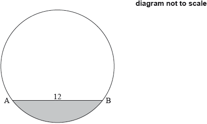
Find the area of the shaded segment.
-
21M.2.SL.TZ2.2b:
Find .
-
21M.2.SL.TZ2.2d:
Estimate . You may assume the highway has a width of zero.
-
17N.2.SL.TZ0.T_3a:
Show that correct to the nearest metre.
-
19M.2.AHL.TZ2.H_1:
In triangle ABC, AB = 5, BC = 14 and AC = 11.
Find all the interior angles of the triangle. Give your answers in degrees to one decimal place.
-
17M.2.AHL.TZ1.H_10b:
Calculate the two corresponding values of PQ.
-
17M.2.SL.TZ1.T_2c:
Show that angle , correct to one decimal place.
-
19N.2.SL.TZ0.T_2f:
Given that the length of is , find the area of triangle .
-
17M.2.AHL.TZ1.H_10d:
Determine the range of values of for which it is possible to form two triangles.
-
20N.2.SL.TZ0.T_3a:
Calculate the length of .
-
EXN.1.SL.TZ0.11a:
Find the area of the field.
-
EXN.1.SL.TZ0.11b:
The farmer would like to divide the field into two equal parts by constructing a straight fence from to a point on .
Find . Fully justify any assumptions you make.
-
21M.1.SL.TZ2.9a:
A footpath is to be laid around the curved side of the lawn. Find the length of the footpath.
-
21M.1.SL.TZ1.9:
A triangular field is such that and , each measured correct to the nearest metre, and the angle at is equal to , measured correct to the nearest .

Calculate the maximum possible area of the field.
-
21M.1.SL.TZ2.9b:
Find the area of the lawn.
-
21M.2.SL.TZ2.2a:
Find the size of .
-
21M.2.SL.TZ2.5a:
Given that , show that the area of the base of the box is equal to .
-
21N.1.AHL.TZ0.11:
The following diagram shows a corner of a field bounded by two walls defined by lines and . The walls meet at a point , making an angle of .
Farmer Nate has of fencing to make a triangular enclosure for his sheep. One end of the fence is positioned at a point on , from . The other end of the fence will be positioned at some point on , as shown on the diagram.

He wants the enclosure to take up as little of the current field as possible.
Find the minimum possible area of the triangular enclosure .
-
21N.2.SL.TZ0.4a:
Find the angle of depression from to .
-
21N.2.SL.TZ0.4b.i:
Find .
-
21N.2.SL.TZ0.4c:
By finding an appropriate value, determine whether Joshua is correct.
-
21N.2.SL.TZ0.4d:
To avoid water leaking into the ground, the five interior sides of the reservoir have been painted with a watertight material.
Find the area that was painted.
-
21N.1.SL.TZ0.2a:
Calculate the value of , the measure of angle .