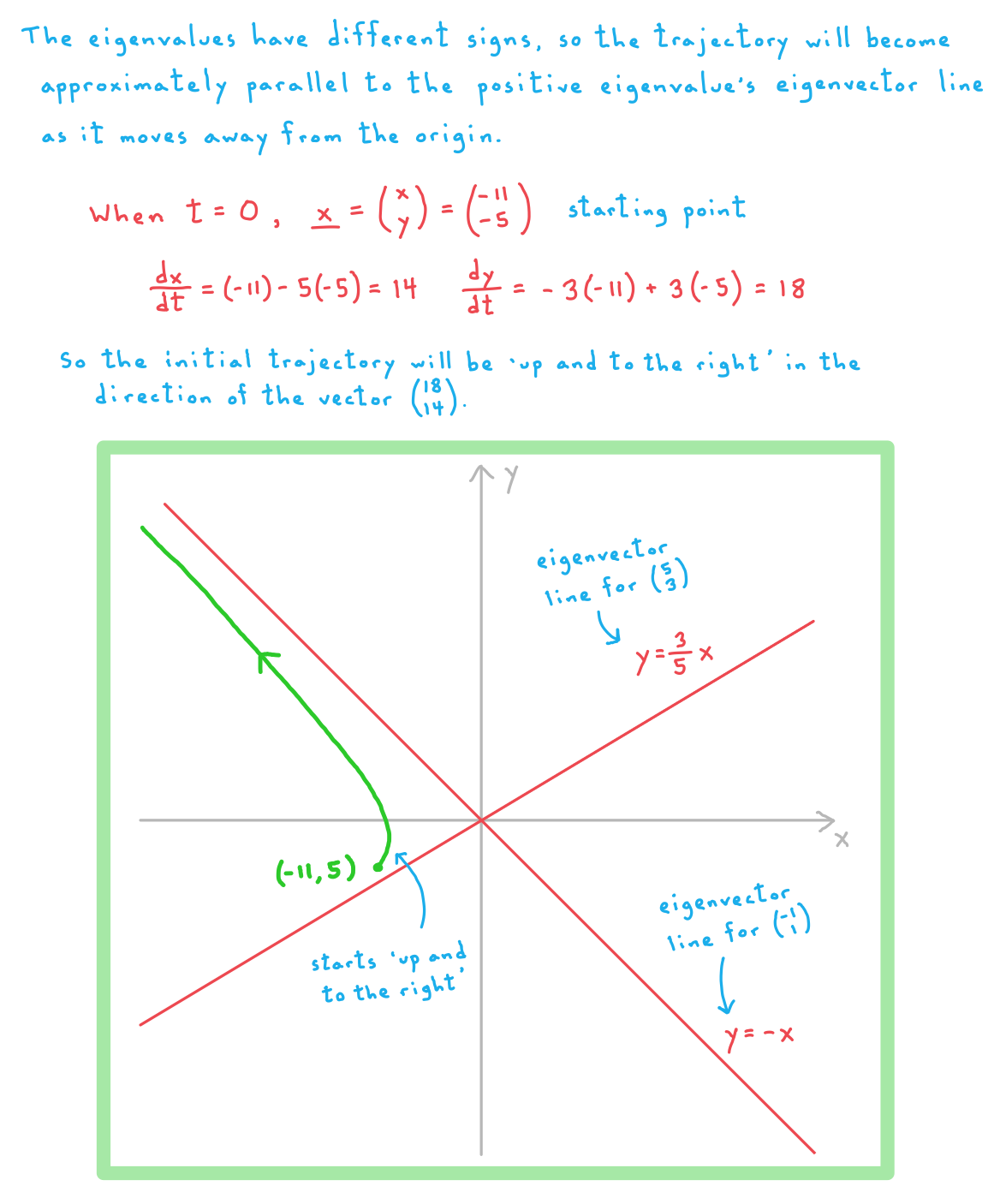
Solving Coupled Differential Equations
How do I write a system of coupled differential equations in matrix form?
- The coupled differential equations considered in this part of the course will be of the form
format('truetype')%3Bfont-weight%3Anormal%3Bfont-style%3Anormal%3B%7D%3C%2Fstyle%3E%3C%2Fdefs%3E%3Cline%20stroke%3D%22%23000000%22%20stroke-linecap%3D%22square%22%20stroke-width%3D%221%22%20x1%3D%222.5%22%20x2%3D%2225.5%22%20y1%3D%2223.5%22%20y2%3D%2223.5%22%2F%3E%3Ctext%20font-family%3D%22Times%20New%20Roman%22%20font-size%3D%2218%22%20text-anchor%3D%22middle%22%20x%3D%229.5%22%20y%3D%2216%22%3Ed%3C%2Ftext%3E%3Ctext%20font-family%3D%22Times%20New%20Roman%22%20font-size%3D%2218%22%20font-style%3D%22italic%22%20text-anchor%3D%22middle%22%20x%3D%2218.5%22%20y%3D%2216%22%3Ex%3C%2Ftext%3E%3Ctext%20font-family%3D%22Times%20New%20Roman%22%20font-size%3D%2218%22%20text-anchor%3D%22middle%22%20x%3D%2211.5%22%20y%3D%2241%22%3Ed%3C%2Ftext%3E%3Ctext%20font-family%3D%22Times%20New%20Roman%22%20font-size%3D%2218%22%20font-style%3D%22italic%22%20text-anchor%3D%22middle%22%20x%3D%2218.5%22%20y%3D%2241%22%3Et%3C%2Ftext%3E%3Ctext%20font-family%3D%22math1564b4c0e54101ac57a0cb68c16%22%20font-size%3D%2216%22%20text-anchor%3D%22middle%22%20x%3D%2236.5%22%20y%3D%2230%22%3E%3D%3C%2Ftext%3E%3Ctext%20font-family%3D%22Times%20New%20Roman%22%20font-size%3D%2218%22%20font-style%3D%22italic%22%20text-anchor%3D%22middle%22%20x%3D%2249.5%22%20y%3D%2230%22%3Ea%3C%2Ftext%3E%3Ctext%20font-family%3D%22Times%20New%20Roman%22%20font-size%3D%2218%22%20font-style%3D%22italic%22%20text-anchor%3D%22middle%22%20x%3D%2257.5%22%20y%3D%2230%22%3Ex%3C%2Ftext%3E%3Ctext%20font-family%3D%22math1564b4c0e54101ac57a0cb68c16%22%20font-size%3D%2216%22%20text-anchor%3D%22middle%22%20x%3D%2271.5%22%20y%3D%2230%22%3E%2B%3C%2Ftext%3E%3Ctext%20font-family%3D%22Times%20New%20Roman%22%20font-size%3D%2218%22%20font-style%3D%22italic%22%20text-anchor%3D%22middle%22%20x%3D%2284.5%22%20y%3D%2230%22%3Eb%3C%2Ftext%3E%3Ctext%20font-family%3D%22Times%20New%20Roman%22%20font-size%3D%2218%22%20font-style%3D%22italic%22%20text-anchor%3D%22middle%22%20x%3D%2293.5%22%20y%3D%2230%22%3Ey%3C%2Ftext%3E%3C%2Fsvg%3E)
format('truetype')%3Bfont-weight%3Anormal%3Bfont-style%3Anormal%3B%7D%3C%2Fstyle%3E%3C%2Fdefs%3E%3Cline%20stroke%3D%22%23000000%22%20stroke-linecap%3D%22square%22%20stroke-width%3D%221%22%20x1%3D%222.5%22%20x2%3D%2225.5%22%20y1%3D%2223.5%22%20y2%3D%2223.5%22%2F%3E%3Ctext%20font-family%3D%22Times%20New%20Roman%22%20font-size%3D%2218%22%20text-anchor%3D%22middle%22%20x%3D%229.5%22%20y%3D%2216%22%3Ed%3C%2Ftext%3E%3Ctext%20font-family%3D%22Times%20New%20Roman%22%20font-size%3D%2218%22%20font-style%3D%22italic%22%20text-anchor%3D%22middle%22%20x%3D%2218.5%22%20y%3D%2216%22%3Ey%3C%2Ftext%3E%3Ctext%20font-family%3D%22Times%20New%20Roman%22%20font-size%3D%2218%22%20text-anchor%3D%22middle%22%20x%3D%2211.5%22%20y%3D%2241%22%3Ed%3C%2Ftext%3E%3Ctext%20font-family%3D%22Times%20New%20Roman%22%20font-size%3D%2218%22%20font-style%3D%22italic%22%20text-anchor%3D%22middle%22%20x%3D%2218.5%22%20y%3D%2241%22%3Et%3C%2Ftext%3E%3Ctext%20font-family%3D%22math1564b4c0e54101ac57a0cb68c16%22%20font-size%3D%2216%22%20text-anchor%3D%22middle%22%20x%3D%2236.5%22%20y%3D%2230%22%3E%3D%3C%2Ftext%3E%3Ctext%20font-family%3D%22Times%20New%20Roman%22%20font-size%3D%2218%22%20font-style%3D%22italic%22%20text-anchor%3D%22middle%22%20x%3D%2249.5%22%20y%3D%2230%22%3Ec%3C%2Ftext%3E%3Ctext%20font-family%3D%22Times%20New%20Roman%22%20font-size%3D%2218%22%20font-style%3D%22italic%22%20text-anchor%3D%22middle%22%20x%3D%2257.5%22%20y%3D%2230%22%3Ex%3C%2Ftext%3E%3Ctext%20font-family%3D%22math1564b4c0e54101ac57a0cb68c16%22%20font-size%3D%2216%22%20text-anchor%3D%22middle%22%20x%3D%2271.5%22%20y%3D%2230%22%3E%2B%3C%2Ftext%3E%3Ctext%20font-family%3D%22Times%20New%20Roman%22%20font-size%3D%2218%22%20font-style%3D%22italic%22%20text-anchor%3D%22middle%22%20x%3D%2284.5%22%20y%3D%2230%22%3Ed%3C%2Ftext%3E%3Ctext%20font-family%3D%22Times%20New%20Roman%22%20font-size%3D%2218%22%20font-style%3D%22italic%22%20text-anchor%3D%22middle%22%20x%3D%2293.5%22%20y%3D%2230%22%3Ey%3C%2Ftext%3E%3C%2Fsvg%3E)
-
-
format('truetype')%3Bfont-weight%3Anormal%3Bfont-style%3Anormal%3B%7D%3C%2Fstyle%3E%3C%2Fdefs%3E%3Ctext%20font-family%3D%22Times%20New%20Roman%22%20font-size%3D%2218%22%20font-style%3D%22italic%22%20text-anchor%3D%22middle%22%20x%3D%224.5%22%20y%3D%2216%22%3Ea%3C%2Ftext%3E%3Ctext%20font-family%3D%22math1c4e7e3cc37e8917655f7289e07%22%20font-size%3D%2216%22%20text-anchor%3D%22middle%22%20x%3D%2211.5%22%20y%3D%2216%22%3E%2C%3C%2Ftext%3E%3Ctext%20font-family%3D%22Times%20New%20Roman%22%20font-size%3D%2218%22%20font-style%3D%22italic%22%20text-anchor%3D%22middle%22%20x%3D%2222.5%22%20y%3D%2216%22%3Eb%3C%2Ftext%3E%3Ctext%20font-family%3D%22math1c4e7e3cc37e8917655f7289e07%22%20font-size%3D%2216%22%20text-anchor%3D%22middle%22%20x%3D%2230.5%22%20y%3D%2216%22%3E%2C%3C%2Ftext%3E%3Ctext%20font-family%3D%22Times%20New%20Roman%22%20font-size%3D%2218%22%20font-style%3D%22italic%22%20text-anchor%3D%22middle%22%20x%3D%2241.5%22%20y%3D%2216%22%3Ec%3C%2Ftext%3E%3Ctext%20font-family%3D%22math1c4e7e3cc37e8917655f7289e07%22%20font-size%3D%2216%22%20text-anchor%3D%22middle%22%20x%3D%2248.5%22%20y%3D%2216%22%3E%2C%3C%2Ftext%3E%3Ctext%20font-family%3D%22Times%20New%20Roman%22%20font-size%3D%2218%22%20font-style%3D%22italic%22%20text-anchor%3D%22middle%22%20x%3D%2259.5%22%20y%3D%2216%22%3Ed%3C%2Ftext%3E%3Ctext%20font-family%3D%22math1c4e7e3cc37e8917655f7289e07%22%20font-size%3D%2216%22%20text-anchor%3D%22middle%22%20x%3D%2277.5%22%20y%3D%2216%22%3E%26%23x2208%3B%3C%2Ftext%3E%3Ctext%20font-family%3D%22math1c4e7e3cc37e8917655f7289e07%22%20font-size%3D%2216%22%20text-anchor%3D%22middle%22%20x%3D%2295.5%22%20y%3D%2216%22%3E%26%23x211D%3B%3C%2Ftext%3E%3C%2Fsvg%3E) are constants whose precise value will depend on the situation being modelled
are constants whose precise value will depend on the situation being modelled
- In an exam question the values of the constants will generally be given to you
-
- This system of equations can also be represented in matrix form:
format('truetype')%3Bfont-weight%3Anormal%3Bfont-style%3Anormal%3B%7D%40font-face%7Bfont-family%3A'brack_sm2882ad605b1e27be87c7468'%3Bsrc%3Aurl(data%3Afont%2Ftruetype%3Bcharset%3Dutf-8%3Bbase64%2CAAEAAAAMAIAAAwBAT1MvMi7PH4UAAADMAAAATmNtYXA3kjw6AAABHAAAADxjdnQgAQYDiAAAAVgAAAASZ2x5ZkyYQ7YAAAFsAAAAkWhlYWQLyR8fAAACAAAAADZoaGVhAq0XCAAAAjgAAAAkaG10eDEjA%2FUAAAJcAAAADGxvY2EAAEKZAAACaAAAABBtYXhwBJsEcQAAAngAAAAgbmFtZW7QvZAAAAKYAAAB5XBvc3QArQBVAAAEgAAAACBwcmVwu5WEAAAABKAAAAAHAAACDAGQAAUAAAQABAAAAAAABAAEAAAAAAAAAQEAAAAAAAAAAAAAAAAAAAAAAAAAAAAAAAAAAAAAACAgICAAAAAg9AMD%2FP%2F8AAABVAABAAAAAAACAAEAAQAAABQAAwABAAAAFAAEACgAAAAGAAQAAQACI5wjn%2F%2F%2FAAAjnCOf%2F%2F%2FcZdxjAAEAAAAAAAAAAAFUAFQBAAArAIwAgACoAAcAAAACAAAAAADVAQEAAwAHAAAxMxEjFyM1M9XVq4CAAQHWqwABAAAAAABVAVgAAwAfGAGwAy%2BwADyxAgL1sAE8ALEDAD%2BwAjx8sQAG9bABPBEzESNVVQFY%2FqgAAQDXAAABLAFUAAMAIBgBsAUvsAE8sAI8sQAC9bADPACwAy%2BwAjyxAAH1sAE8EzMRI9dVVQFU%2FqwAAAAAAQAAAAEAAIsesexfDzz1AAMEAP%2F%2F%2F%2F%2FVre5k%2F%2F%2F%2F%2F9Wt7mT%2FgP%2F%2FAdYBWAAAAAoAAgABAAAAAAABAAABVP%2F%2FAAAXcP%2BA%2F4AB1gABAAAAAAAAAAAAAAAAAAAAAwDVAAABLAAAASwA1wAAAAAAAAAhAAAAWAAAAJEAAQAAAAMACgACAAAAAAACAIAEAAAAAAAEAABlAAAAAAAAABUBAgAAAAAAAAABACYAAAAAAAAAAAACAA4AJgAAAAAAAAADAEQANAAAAAAAAAAEACYAeAAAAAAAAAAFABYAngAAAAAAAAAGABMAtAAAAAAAAAAIABwAxwABAAAAAAABACYAAAABAAAAAAACAA4AJgABAAAAAAADAEQANAABAAAAAAAEACYAeAABAAAAAAAFABYAngABAAAAAAAGABMAtAABAAAAAAAIABwAxwADAAEECQABACYAAAADAAEECQACAA4AJgADAAEECQADAEQANAADAAEECQAEACYAeAADAAEECQAFABYAngADAAEECQAGABMAtAADAAEECQAIABwAxwBCAHIAYQBjAGsAZQB0AHMAIABzAG0AYQBsAGwAIABzAGkAegBlAFIAZQBnAHUAbABhAHIATQBhAHQAaABzACAARgBvAHIAIABNAG8AcgBlACAAQgByAGEAYwBrAGUAdABzACAAcwBtAGEAbABsACAAcwBpAHoAZQBCAHIAYQBjAGsAZQB0AHMAIABzAG0AYQBsAGwAIABzAGkAegBlAFYAZQByAHMAaQBvAG4AIAAyAC4AMEJyYWNrZXRzX3NtYWxsX3NpemUATQBhAHQAaABzACAARgBvAHIAIABNAG8AcgBlAAAAAAMAAAAAAAAAqgBVAAAAAAAAAAAAAAAAAAAAAAAAAAC5B%2F8AAo2FAA%3D%3D)format('truetype')%3Bfont-weight%3Anormal%3Bfont-style%3Anormal%3B%7D%40font-face%7Bfont-family%3A'bracketse552f5417ff4680c6b50499'%3Bsrc%3Aurl(data%3Afont%2Ftruetype%3Bcharset%3Dutf-8%3Bbase64%2CAAEAAAAMAIAAAwBAT1MvMi7RIisAAADMAAAATmNtYXBi7uzYAAABHAAAAExjdnQgBAkDLgAAAWgAAAASZ2x5Zo64f%2BkAAAF8AAABSWhlYWQLniGcAAACyAAAADZoaGVhBK4XLAAAAwAAAAAkaG10eCWq%2F90AAAMkAAAAFGxvY2EAABknAAADOAAAABhtYXhwBJIESAAAA1AAAAAgbmFtZRAA8I4AAANwAAAB3nBvc3QBwwDgAAAFUAAAACBwcmVwupWEAAAABXAAAAAHAAACggGQAAUAAAQABAAAAAAABAAEAAAAAAAAAQEAAAAAAAAAAAAAAAAAAAAAAAAAAAAAAAAAAAAAACAgICAAAAAg9AMEAAAAAAADgAAAAAAAAAACAAEAAQAAABQAAwABAAAAFAAEADgAAAAKAAgAAgACI5sjnSOeI6D%2F%2FwAAI5sjnSOeI6D%2F%2F9xm3GXcZdxkAAEAAAAAAAAAAAAAAAABVABWAQAALACoA4AAMgAHAAAAAgAAACoA1QNVAAMABwAANTMRIxMjETPV1auAgCoDK%2F0AAtUAAQAAAAABgAOAAAUAJBgBsAAvsAPFsQEC%2FbADELEEBP0AsQAAP7ABPLEEBj%2BwAzwwMTEzEAEjAFUBKyv%2BqwH8AYT%2BqgABAAAAAAGAA4AABQAmGAGwAC6wA8WxBQL9sAMQsQIE%2FQB8sQAGPxiwBTyxAwb2sAI8MDEREgEzABMBAVQr%2FtMCA4D91v6qAYQB%2FAAB%2F6wAAAEsA4AABQAnGAGwAC%2BwBzywA8WxAQL9sAMQsQQE%2FQCxAAA%2FsAE8sQQGP7ADPDAxISMSATMAASxVAf7UKwFVAfwBhP6rAAH%2FrAAAASwDgAAFACkYAbABL7AHPLAExbEAAv2wBBCxAwT9AHyxAQY%2FsAA8GLEEAD%2BwAzwwMRMzEAEjANdV%2FqsrASsDgP3V%2FqsBhgAAAAABAAAAAQAAeuTcpl8PPPUAAwQA%2F%2F%2F%2F%2F9Wt7o7%2F%2F%2F%2F%2F1a3ujv%2BsAAABgAOAAAAACgACAAEAAAAAAAEAAAOAAAAAABdw%2F6z%2FrAGAAAEAAAAAAAAAAAAAAAAAAAAFANUAAAEsAAABLAAAASz%2FrAEs%2F6wAAAAAAAAAJAAAAGgAAACzAAAA%2FQAAAUkAAQAAAAUACAACAAAAAAACAIAEAAAAAAAEAAA%2BAAAAAAAAABUBAgAAAAAAAAABACQAAAAAAAAAAAACAA4AJAAAAAAAAAADAEIAMgAAAAAAAAAEACQAdAAAAAAAAAAFABYAmAAAAAAAAAAGABIArgAAAAAAAAAIABwAwAABAAAAAAABACQAAAABAAAAAAACAA4AJAABAAAAAAADAEIAMgABAAAAAAAEACQAdAABAAAAAAAFABYAmAABAAAAAAAGABIArgABAAAAAAAIABwAwAADAAEECQABACQAAAADAAEECQACAA4AJAADAAEECQADAEIAMgADAAEECQAEACQAdAADAAEECQAFABYAmAADAAEECQAGABIArgADAAEECQAIABwAwABCAHIAYQBjAGsAZQB0AHMAIABmAHUAbABsACAAcwBpAHoAZQBSAGUAZwB1AGwAYQByAE0AYQB0AGgAcwAgAEYAbwByACAATQBvAHIAZQAgAEIAcgBhAGMAawBlAHQAcwAgAGYAdQBsAGwAIABzAGkAegBlAEIAcgBhAGMAawBlAHQAcwAgAGYAdQBsAGwAIABzAGkAegBlAFYAZQByAHMAaQBvAG4AIAAyAC4AMEJyYWNrZXRzX2Z1bGxfc2l6ZQBNAGEAdABoAHMAIABGAG8AcgAgAE0AbwByAGUAAAADAAAAAAAAAcAA4AAAAAAAAAAAAAAAAAAAAAAAAAAAuQf%2FAAGNhQA%3D)format('truetype')%3Bfont-weight%3Anormal%3Bfont-style%3Anormal%3B%7D%3C%2Fstyle%3E%3C%2Fdefs%3E%3Ctext%20font-family%3D%22bracketse552f5417ff4680c6b50499%22%20font-size%3D%2218%22%20text-anchor%3D%22start%22%20x%3D%221.5%22%20y%3D%2219%22%3E%26%23x239B%3B%3C%2Ftext%3E%3Ctext%20font-family%3D%22brack_sm2882ad605b1e27be87c7468%22%20font-size%3D%2218%22%20text-anchor%3D%22start%22%20x%3D%221.5%22%20y%3D%2225%22%3E%26%23x239C%3B%3C%2Ftext%3E%3Ctext%20font-family%3D%22brack_sm2882ad605b1e27be87c7468%22%20font-size%3D%2218%22%20text-anchor%3D%22start%22%20x%3D%221.5%22%20y%3D%2231%22%3E%26%23x239C%3B%3C%2Ftext%3E%3Ctext%20font-family%3D%22brack_sm2882ad605b1e27be87c7468%22%20font-size%3D%2218%22%20text-anchor%3D%22start%22%20x%3D%221.5%22%20y%3D%2237%22%3E%26%23x239C%3B%3C%2Ftext%3E%3Ctext%20font-family%3D%22brack_sm2882ad605b1e27be87c7468%22%20font-size%3D%2218%22%20text-anchor%3D%22start%22%20x%3D%221.5%22%20y%3D%2243%22%3E%26%23x239C%3B%3C%2Ftext%3E%3Ctext%20font-family%3D%22brack_sm2882ad605b1e27be87c7468%22%20font-size%3D%2218%22%20text-anchor%3D%22start%22%20x%3D%221.5%22%20y%3D%2249%22%3E%26%23x239C%3B%3C%2Ftext%3E%3Ctext%20font-family%3D%22brack_sm2882ad605b1e27be87c7468%22%20font-size%3D%2218%22%20text-anchor%3D%22start%22%20x%3D%221.5%22%20y%3D%2255%22%3E%26%23x239C%3B%3C%2Ftext%3E%3Ctext%20font-family%3D%22brack_sm2882ad605b1e27be87c7468%22%20font-size%3D%2218%22%20text-anchor%3D%22start%22%20x%3D%221.5%22%20y%3D%2261%22%3E%26%23x239C%3B%3C%2Ftext%3E%3Ctext%20font-family%3D%22brack_sm2882ad605b1e27be87c7468%22%20font-size%3D%2218%22%20text-anchor%3D%22start%22%20x%3D%221.5%22%20y%3D%2267%22%3E%26%23x239C%3B%3C%2Ftext%3E%3Ctext%20font-family%3D%22brack_sm2882ad605b1e27be87c7468%22%20font-size%3D%2218%22%20text-anchor%3D%22start%22%20x%3D%221.5%22%20y%3D%2273%22%3E%26%23x239C%3B%3C%2Ftext%3E%3Ctext%20font-family%3D%22brack_sm2882ad605b1e27be87c7468%22%20font-size%3D%2218%22%20text-anchor%3D%22start%22%20x%3D%221.5%22%20y%3D%2279%22%3E%26%23x239C%3B%3C%2Ftext%3E%3Ctext%20font-family%3D%22brack_sm2882ad605b1e27be87c7468%22%20font-size%3D%2218%22%20text-anchor%3D%22start%22%20x%3D%221.5%22%20y%3D%2285%22%3E%26%23x239C%3B%3C%2Ftext%3E%3Ctext%20font-family%3D%22bracketse552f5417ff4680c6b50499%22%20font-size%3D%2218%22%20text-anchor%3D%22start%22%20x%3D%221.5%22%20y%3D%22101%22%3E%26%23x239D%3B%3C%2Ftext%3E%3Ctext%20font-family%3D%22bracketse552f5417ff4680c6b50499%22%20font-size%3D%2218%22%20text-anchor%3D%22start%22%20x%3D%2244.5%22%20y%3D%2219%22%3E%26%23x239E%3B%3C%2Ftext%3E%3Ctext%20font-family%3D%22brack_sm2882ad605b1e27be87c7468%22%20font-size%3D%2218%22%20text-anchor%3D%22start%22%20x%3D%2244.5%22%20y%3D%2225%22%3E%26%23x239F%3B%3C%2Ftext%3E%3Ctext%20font-family%3D%22brack_sm2882ad605b1e27be87c7468%22%20font-size%3D%2218%22%20text-anchor%3D%22start%22%20x%3D%2244.5%22%20y%3D%2231%22%3E%26%23x239F%3B%3C%2Ftext%3E%3Ctext%20font-family%3D%22brack_sm2882ad605b1e27be87c7468%22%20font-size%3D%2218%22%20text-anchor%3D%22start%22%20x%3D%2244.5%22%20y%3D%2237%22%3E%26%23x239F%3B%3C%2Ftext%3E%3Ctext%20font-family%3D%22brack_sm2882ad605b1e27be87c7468%22%20font-size%3D%2218%22%20text-anchor%3D%22start%22%20x%3D%2244.5%22%20y%3D%2243%22%3E%26%23x239F%3B%3C%2Ftext%3E%3Ctext%20font-family%3D%22brack_sm2882ad605b1e27be87c7468%22%20font-size%3D%2218%22%20text-anchor%3D%22start%22%20x%3D%2244.5%22%20y%3D%2249%22%3E%26%23x239F%3B%3C%2Ftext%3E%3Ctext%20font-family%3D%22brack_sm2882ad605b1e27be87c7468%22%20font-size%3D%2218%22%20text-anchor%3D%22start%22%20x%3D%2244.5%22%20y%3D%2255%22%3E%26%23x239F%3B%3C%2Ftext%3E%3Ctext%20font-family%3D%22brack_sm2882ad605b1e27be87c7468%22%20font-size%3D%2218%22%20text-anchor%3D%22start%22%20x%3D%2244.5%22%20y%3D%2261%22%3E%26%23x239F%3B%3C%2Ftext%3E%3Ctext%20font-family%3D%22brack_sm2882ad605b1e27be87c7468%22%20font-size%3D%2218%22%20text-anchor%3D%22start%22%20x%3D%2244.5%22%20y%3D%2267%22%3E%26%23x239F%3B%3C%2Ftext%3E%3Ctext%20font-family%3D%22brack_sm2882ad605b1e27be87c7468%22%20font-size%3D%2218%22%20text-anchor%3D%22start%22%20x%3D%2244.5%22%20y%3D%2273%22%3E%26%23x239F%3B%3C%2Ftext%3E%3Ctext%20font-family%3D%22brack_sm2882ad605b1e27be87c7468%22%20font-size%3D%2218%22%20text-anchor%3D%22start%22%20x%3D%2244.5%22%20y%3D%2279%22%3E%26%23x239F%3B%3C%2Ftext%3E%3Ctext%20font-family%3D%22brack_sm2882ad605b1e27be87c7468%22%20font-size%3D%2218%22%20text-anchor%3D%22start%22%20x%3D%2244.5%22%20y%3D%2285%22%3E%26%23x239F%3B%3C%2Ftext%3E%3Ctext%20font-family%3D%22bracketse552f5417ff4680c6b50499%22%20font-size%3D%2218%22%20text-anchor%3D%22start%22%20x%3D%2244.5%22%20y%3D%22101%22%3E%26%23x23A0%3B%3C%2Ftext%3E%3Cline%20stroke%3D%22%23000000%22%20stroke-linecap%3D%22square%22%20stroke-width%3D%221%22%20x1%3D%2213.5%22%20x2%3D%2236.5%22%20y1%3D%2226.5%22%20y2%3D%2226.5%22%2F%3E%3Ctext%20font-family%3D%22Times%20New%20Roman%22%20font-size%3D%2218%22%20text-anchor%3D%22middle%22%20x%3D%2220.5%22%20y%3D%2219%22%3Ed%3C%2Ftext%3E%3Ctext%20font-family%3D%22Times%20New%20Roman%22%20font-size%3D%2218%22%20font-style%3D%22italic%22%20text-anchor%3D%22middle%22%20x%3D%2229.5%22%20y%3D%2219%22%3Ex%3C%2Ftext%3E%3Ctext%20font-family%3D%22Times%20New%20Roman%22%20font-size%3D%2218%22%20text-anchor%3D%22middle%22%20x%3D%2222.5%22%20y%3D%2244%22%3Ed%3C%2Ftext%3E%3Ctext%20font-family%3D%22Times%20New%20Roman%22%20font-size%3D%2218%22%20font-style%3D%22italic%22%20text-anchor%3D%22middle%22%20x%3D%2229.5%22%20y%3D%2244%22%3Et%3C%2Ftext%3E%3Cline%20stroke%3D%22%23000000%22%20stroke-linecap%3D%22square%22%20stroke-width%3D%221%22%20x1%3D%2213.5%22%20x2%3D%2236.5%22%20y1%3D%2277.5%22%20y2%3D%2277.5%22%2F%3E%3Ctext%20font-family%3D%22Times%20New%20Roman%22%20font-size%3D%2218%22%20text-anchor%3D%22middle%22%20x%3D%2220.5%22%20y%3D%2270%22%3Ed%3C%2Ftext%3E%3Ctext%20font-family%3D%22Times%20New%20Roman%22%20font-size%3D%2218%22%20font-style%3D%22italic%22%20text-anchor%3D%22middle%22%20x%3D%2229.5%22%20y%3D%2270%22%3Ey%3C%2Ftext%3E%3Ctext%20font-family%3D%22Times%20New%20Roman%22%20font-size%3D%2218%22%20text-anchor%3D%22middle%22%20x%3D%2222.5%22%20y%3D%2295%22%3Ed%3C%2Ftext%3E%3Ctext%20font-family%3D%22Times%20New%20Roman%22%20font-size%3D%2218%22%20font-style%3D%22italic%22%20text-anchor%3D%22middle%22%20x%3D%2229.5%22%20y%3D%2295%22%3Et%3C%2Ftext%3E%3Ctext%20font-family%3D%22math17f39f8317fbdb1988ef4c628eb%22%20font-size%3D%2216%22%20text-anchor%3D%22middle%22%20x%3D%2258.5%22%20y%3D%2258%22%3E%3D%3C%2Ftext%3E%3Ctext%20font-family%3D%22bracketse552f5417ff4680c6b50499%22%20font-size%3D%2218%22%20text-anchor%3D%22start%22%20x%3D%2268.5%22%20y%3D%2243%22%3E%26%23x239B%3B%3C%2Ftext%3E%3Ctext%20font-family%3D%22brack_sm2882ad605b1e27be87c7468%22%20font-size%3D%2218%22%20text-anchor%3D%22start%22%20x%3D%2268.5%22%20y%3D%2249%22%3E%26%23x239C%3B%3C%2Ftext%3E%3Ctext%20font-family%3D%22brack_sm2882ad605b1e27be87c7468%22%20font-size%3D%2218%22%20text-anchor%3D%22start%22%20x%3D%2268.5%22%20y%3D%2255%22%3E%26%23x239C%3B%3C%2Ftext%3E%3Ctext%20font-family%3D%22brack_sm2882ad605b1e27be87c7468%22%20font-size%3D%2218%22%20text-anchor%3D%22start%22%20x%3D%2268.5%22%20y%3D%2261%22%3E%26%23x239C%3B%3C%2Ftext%3E%3Ctext%20font-family%3D%22bracketse552f5417ff4680c6b50499%22%20font-size%3D%2218%22%20text-anchor%3D%22start%22%20x%3D%2268.5%22%20y%3D%2277%22%3E%26%23x239D%3B%3C%2Ftext%3E%3Ctext%20font-family%3D%22bracketse552f5417ff4680c6b50499%22%20font-size%3D%2218%22%20text-anchor%3D%22start%22%20x%3D%22110.5%22%20y%3D%2243%22%3E%26%23x239E%3B%3C%2Ftext%3E%3Ctext%20font-family%3D%22brack_sm2882ad605b1e27be87c7468%22%20font-size%3D%2218%22%20text-anchor%3D%22start%22%20x%3D%22110.5%22%20y%3D%2249%22%3E%26%23x239F%3B%3C%2Ftext%3E%3Ctext%20font-family%3D%22brack_sm2882ad605b1e27be87c7468%22%20font-size%3D%2218%22%20text-anchor%3D%22start%22%20x%3D%22110.5%22%20y%3D%2255%22%3E%26%23x239F%3B%3C%2Ftext%3E%3Ctext%20font-family%3D%22brack_sm2882ad605b1e27be87c7468%22%20font-size%3D%2218%22%20text-anchor%3D%22start%22%20x%3D%22110.5%22%20y%3D%2261%22%3E%26%23x239F%3B%3C%2Ftext%3E%3Ctext%20font-family%3D%22bracketse552f5417ff4680c6b50499%22%20font-size%3D%2218%22%20text-anchor%3D%22start%22%20x%3D%22110.5%22%20y%3D%2277%22%3E%26%23x23A0%3B%3C%2Ftext%3E%3Ctext%20font-family%3D%22Times%20New%20Roman%22%20font-size%3D%2218%22%20font-style%3D%22italic%22%20text-anchor%3D%22middle%22%20x%3D%2282.5%22%20y%3D%2244%22%3Ea%3C%2Ftext%3E%3Ctext%20font-family%3D%22Times%20New%20Roman%22%20font-size%3D%2218%22%20font-style%3D%22italic%22%20text-anchor%3D%22middle%22%20x%3D%2299.5%22%20y%3D%2244%22%3Eb%3C%2Ftext%3E%3Ctext%20font-family%3D%22Times%20New%20Roman%22%20font-size%3D%2218%22%20font-style%3D%22italic%22%20text-anchor%3D%22middle%22%20x%3D%2282.5%22%20y%3D%2270%22%3Ec%3C%2Ftext%3E%3Ctext%20font-family%3D%22Times%20New%20Roman%22%20font-size%3D%2218%22%20font-style%3D%22italic%22%20text-anchor%3D%22middle%22%20x%3D%2299.5%22%20y%3D%2270%22%3Ed%3C%2Ftext%3E%3Ctext%20font-family%3D%22bracketse552f5417ff4680c6b50499%22%20font-size%3D%2218%22%20text-anchor%3D%22start%22%20x%3D%22117.5%22%20y%3D%2243%22%3E%26%23x239B%3B%3C%2Ftext%3E%3Ctext%20font-family%3D%22brack_sm2882ad605b1e27be87c7468%22%20font-size%3D%2218%22%20text-anchor%3D%22start%22%20x%3D%22117.5%22%20y%3D%2249%22%3E%26%23x239C%3B%3C%2Ftext%3E%3Ctext%20font-family%3D%22brack_sm2882ad605b1e27be87c7468%22%20font-size%3D%2218%22%20text-anchor%3D%22start%22%20x%3D%22117.5%22%20y%3D%2255%22%3E%26%23x239C%3B%3C%2Ftext%3E%3Ctext%20font-family%3D%22brack_sm2882ad605b1e27be87c7468%22%20font-size%3D%2218%22%20text-anchor%3D%22start%22%20x%3D%22117.5%22%20y%3D%2261%22%3E%26%23x239C%3B%3C%2Ftext%3E%3Ctext%20font-family%3D%22bracketse552f5417ff4680c6b50499%22%20font-size%3D%2218%22%20text-anchor%3D%22start%22%20x%3D%22117.5%22%20y%3D%2277%22%3E%26%23x239D%3B%3C%2Ftext%3E%3Ctext%20font-family%3D%22bracketse552f5417ff4680c6b50499%22%20font-size%3D%2218%22%20text-anchor%3D%22start%22%20x%3D%22142.5%22%20y%3D%2243%22%3E%26%23x239E%3B%3C%2Ftext%3E%3Ctext%20font-family%3D%22brack_sm2882ad605b1e27be87c7468%22%20font-size%3D%2218%22%20text-anchor%3D%22start%22%20x%3D%22142.5%22%20y%3D%2249%22%3E%26%23x239F%3B%3C%2Ftext%3E%3Ctext%20font-family%3D%22brack_sm2882ad605b1e27be87c7468%22%20font-size%3D%2218%22%20text-anchor%3D%22start%22%20x%3D%22142.5%22%20y%3D%2255%22%3E%26%23x239F%3B%3C%2Ftext%3E%3Ctext%20font-family%3D%22brack_sm2882ad605b1e27be87c7468%22%20font-size%3D%2218%22%20text-anchor%3D%22start%22%20x%3D%22142.5%22%20y%3D%2261%22%3E%26%23x239F%3B%3C%2Ftext%3E%3Ctext%20font-family%3D%22bracketse552f5417ff4680c6b50499%22%20font-size%3D%2218%22%20text-anchor%3D%22start%22%20x%3D%22142.5%22%20y%3D%2277%22%3E%26%23x23A0%3B%3C%2Ftext%3E%3Ctext%20font-family%3D%22Times%20New%20Roman%22%20font-size%3D%2218%22%20font-style%3D%22italic%22%20text-anchor%3D%22middle%22%20x%3D%22131.5%22%20y%3D%2244%22%3Ex%3C%2Ftext%3E%3Ctext%20font-family%3D%22Times%20New%20Roman%22%20font-size%3D%2218%22%20font-style%3D%22italic%22%20text-anchor%3D%22middle%22%20x%3D%22131.5%22%20y%3D%2270%22%3Ey%3C%2Ftext%3E%3C%2Fsvg%3E)
- It is usually more convenient, however, to use the ‘dot notation’ for the derivatives:
format('truetype')%3Bfont-weight%3Anormal%3Bfont-style%3Anormal%3B%7D%40font-face%7Bfont-family%3A'brack_sm2882ad605b1e27be87c7468'%3Bsrc%3Aurl(data%3Afont%2Ftruetype%3Bcharset%3Dutf-8%3Bbase64%2CAAEAAAAMAIAAAwBAT1MvMi7PH4UAAADMAAAATmNtYXA3kjw6AAABHAAAADxjdnQgAQYDiAAAAVgAAAASZ2x5ZkyYQ7YAAAFsAAAAkWhlYWQLyR8fAAACAAAAADZoaGVhAq0XCAAAAjgAAAAkaG10eDEjA%2FUAAAJcAAAADGxvY2EAAEKZAAACaAAAABBtYXhwBJsEcQAAAngAAAAgbmFtZW7QvZAAAAKYAAAB5XBvc3QArQBVAAAEgAAAACBwcmVwu5WEAAAABKAAAAAHAAACDAGQAAUAAAQABAAAAAAABAAEAAAAAAAAAQEAAAAAAAAAAAAAAAAAAAAAAAAAAAAAAAAAAAAAACAgICAAAAAg9AMD%2FP%2F8AAABVAABAAAAAAACAAEAAQAAABQAAwABAAAAFAAEACgAAAAGAAQAAQACI5wjn%2F%2F%2FAAAjnCOf%2F%2F%2FcZdxjAAEAAAAAAAAAAAFUAFQBAAArAIwAgACoAAcAAAACAAAAAADVAQEAAwAHAAAxMxEjFyM1M9XVq4CAAQHWqwABAAAAAABVAVgAAwAfGAGwAy%2BwADyxAgL1sAE8ALEDAD%2BwAjx8sQAG9bABPBEzESNVVQFY%2FqgAAQDXAAABLAFUAAMAIBgBsAUvsAE8sAI8sQAC9bADPACwAy%2BwAjyxAAH1sAE8EzMRI9dVVQFU%2FqwAAAAAAQAAAAEAAIsesexfDzz1AAMEAP%2F%2F%2F%2F%2FVre5k%2F%2F%2F%2F%2F9Wt7mT%2FgP%2F%2FAdYBWAAAAAoAAgABAAAAAAABAAABVP%2F%2FAAAXcP%2BA%2F4AB1gABAAAAAAAAAAAAAAAAAAAAAwDVAAABLAAAASwA1wAAAAAAAAAhAAAAWAAAAJEAAQAAAAMACgACAAAAAAACAIAEAAAAAAAEAABlAAAAAAAAABUBAgAAAAAAAAABACYAAAAAAAAAAAACAA4AJgAAAAAAAAADAEQANAAAAAAAAAAEACYAeAAAAAAAAAAFABYAngAAAAAAAAAGABMAtAAAAAAAAAAIABwAxwABAAAAAAABACYAAAABAAAAAAACAA4AJgABAAAAAAADAEQANAABAAAAAAAEACYAeAABAAAAAAAFABYAngABAAAAAAAGABMAtAABAAAAAAAIABwAxwADAAEECQABACYAAAADAAEECQACAA4AJgADAAEECQADAEQANAADAAEECQAEACYAeAADAAEECQAFABYAngADAAEECQAGABMAtAADAAEECQAIABwAxwBCAHIAYQBjAGsAZQB0AHMAIABzAG0AYQBsAGwAIABzAGkAegBlAFIAZQBnAHUAbABhAHIATQBhAHQAaABzACAARgBvAHIAIABNAG8AcgBlACAAQgByAGEAYwBrAGUAdABzACAAcwBtAGEAbABsACAAcwBpAHoAZQBCAHIAYQBjAGsAZQB0AHMAIABzAG0AYQBsAGwAIABzAGkAegBlAFYAZQByAHMAaQBvAG4AIAAyAC4AMEJyYWNrZXRzX3NtYWxsX3NpemUATQBhAHQAaABzACAARgBvAHIAIABNAG8AcgBlAAAAAAMAAAAAAAAAqgBVAAAAAAAAAAAAAAAAAAAAAAAAAAC5B%2F8AAo2FAA%3D%3D)format('truetype')%3Bfont-weight%3Anormal%3Bfont-style%3Anormal%3B%7D%40font-face%7Bfont-family%3A'bracketse552f5417ff4680c6b50499'%3Bsrc%3Aurl(data%3Afont%2Ftruetype%3Bcharset%3Dutf-8%3Bbase64%2CAAEAAAAMAIAAAwBAT1MvMi7RIisAAADMAAAATmNtYXBi7uzYAAABHAAAAExjdnQgBAkDLgAAAWgAAAASZ2x5Zo64f%2BkAAAF8AAABSWhlYWQLniGcAAACyAAAADZoaGVhBK4XLAAAAwAAAAAkaG10eCWq%2F90AAAMkAAAAFGxvY2EAABknAAADOAAAABhtYXhwBJIESAAAA1AAAAAgbmFtZRAA8I4AAANwAAAB3nBvc3QBwwDgAAAFUAAAACBwcmVwupWEAAAABXAAAAAHAAACggGQAAUAAAQABAAAAAAABAAEAAAAAAAAAQEAAAAAAAAAAAAAAAAAAAAAAAAAAAAAAAAAAAAAACAgICAAAAAg9AMEAAAAAAADgAAAAAAAAAACAAEAAQAAABQAAwABAAAAFAAEADgAAAAKAAgAAgACI5sjnSOeI6D%2F%2FwAAI5sjnSOeI6D%2F%2F9xm3GXcZdxkAAEAAAAAAAAAAAAAAAABVABWAQAALACoA4AAMgAHAAAAAgAAACoA1QNVAAMABwAANTMRIxMjETPV1auAgCoDK%2F0AAtUAAQAAAAABgAOAAAUAJBgBsAAvsAPFsQEC%2FbADELEEBP0AsQAAP7ABPLEEBj%2BwAzwwMTEzEAEjAFUBKyv%2BqwH8AYT%2BqgABAAAAAAGAA4AABQAmGAGwAC6wA8WxBQL9sAMQsQIE%2FQB8sQAGPxiwBTyxAwb2sAI8MDEREgEzABMBAVQr%2FtMCA4D91v6qAYQB%2FAAB%2F6wAAAEsA4AABQAnGAGwAC%2BwBzywA8WxAQL9sAMQsQQE%2FQCxAAA%2FsAE8sQQGP7ADPDAxISMSATMAASxVAf7UKwFVAfwBhP6rAAH%2FrAAAASwDgAAFACkYAbABL7AHPLAExbEAAv2wBBCxAwT9AHyxAQY%2FsAA8GLEEAD%2BwAzwwMRMzEAEjANdV%2FqsrASsDgP3V%2FqsBhgAAAAABAAAAAQAAeuTcpl8PPPUAAwQA%2F%2F%2F%2F%2F9Wt7o7%2F%2F%2F%2F%2F1a3ujv%2BsAAABgAOAAAAACgACAAEAAAAAAAEAAAOAAAAAABdw%2F6z%2FrAGAAAEAAAAAAAAAAAAAAAAAAAAFANUAAAEsAAABLAAAASz%2FrAEs%2F6wAAAAAAAAAJAAAAGgAAACzAAAA%2FQAAAUkAAQAAAAUACAACAAAAAAACAIAEAAAAAAAEAAA%2BAAAAAAAAABUBAgAAAAAAAAABACQAAAAAAAAAAAACAA4AJAAAAAAAAAADAEIAMgAAAAAAAAAEACQAdAAAAAAAAAAFABYAmAAAAAAAAAAGABIArgAAAAAAAAAIABwAwAABAAAAAAABACQAAAABAAAAAAACAA4AJAABAAAAAAADAEIAMgABAAAAAAAEACQAdAABAAAAAAAFABYAmAABAAAAAAAGABIArgABAAAAAAAIABwAwAADAAEECQABACQAAAADAAEECQACAA4AJAADAAEECQADAEIAMgADAAEECQAEACQAdAADAAEECQAFABYAmAADAAEECQAGABIArgADAAEECQAIABwAwABCAHIAYQBjAGsAZQB0AHMAIABmAHUAbABsACAAcwBpAHoAZQBSAGUAZwB1AGwAYQByAE0AYQB0AGgAcwAgAEYAbwByACAATQBvAHIAZQAgAEIAcgBhAGMAawBlAHQAcwAgAGYAdQBsAGwAIABzAGkAegBlAEIAcgBhAGMAawBlAHQAcwAgAGYAdQBsAGwAIABzAGkAegBlAFYAZQByAHMAaQBvAG4AIAAyAC4AMEJyYWNrZXRzX2Z1bGxfc2l6ZQBNAGEAdABoAHMAIABGAG8AcgAgAE0AbwByAGUAAAADAAAAAAAAAcAA4AAAAAAAAAAAAAAAAAAAAAAAAAAAuQf%2FAAGNhQA%3D)format('truetype')%3Bfont-weight%3Anormal%3Bfont-style%3Anormal%3B%7D%3C%2Fstyle%3E%3C%2Fdefs%3E%3Ctext%20font-family%3D%22bracketse552f5417ff4680c6b50499%22%20font-size%3D%2218%22%20text-anchor%3D%22start%22%20x%3D%221.5%22%20y%3D%2217%22%3E%26%23x239B%3B%3C%2Ftext%3E%3Ctext%20font-family%3D%22brack_sm2882ad605b1e27be87c7468%22%20font-size%3D%2218%22%20text-anchor%3D%22start%22%20x%3D%221.5%22%20y%3D%2223%22%3E%26%23x239C%3B%3C%2Ftext%3E%3Ctext%20font-family%3D%22brack_sm2882ad605b1e27be87c7468%22%20font-size%3D%2218%22%20text-anchor%3D%22start%22%20x%3D%221.5%22%20y%3D%2229%22%3E%26%23x239C%3B%3C%2Ftext%3E%3Ctext%20font-family%3D%22brack_sm2882ad605b1e27be87c7468%22%20font-size%3D%2218%22%20text-anchor%3D%22start%22%20x%3D%221.5%22%20y%3D%2235%22%3E%26%23x239C%3B%3C%2Ftext%3E%3Ctext%20font-family%3D%22brack_sm2882ad605b1e27be87c7468%22%20font-size%3D%2218%22%20text-anchor%3D%22start%22%20x%3D%221.5%22%20y%3D%2241%22%3E%26%23x239C%3B%3C%2Ftext%3E%3Ctext%20font-family%3D%22bracketse552f5417ff4680c6b50499%22%20font-size%3D%2218%22%20text-anchor%3D%22start%22%20x%3D%221.5%22%20y%3D%2257%22%3E%26%23x239D%3B%3C%2Ftext%3E%3Ctext%20font-family%3D%22bracketse552f5417ff4680c6b50499%22%20font-size%3D%2218%22%20text-anchor%3D%22start%22%20x%3D%2226.5%22%20y%3D%2217%22%3E%26%23x239E%3B%3C%2Ftext%3E%3Ctext%20font-family%3D%22brack_sm2882ad605b1e27be87c7468%22%20font-size%3D%2218%22%20text-anchor%3D%22start%22%20x%3D%2226.5%22%20y%3D%2223%22%3E%26%23x239F%3B%3C%2Ftext%3E%3Ctext%20font-family%3D%22brack_sm2882ad605b1e27be87c7468%22%20font-size%3D%2218%22%20text-anchor%3D%22start%22%20x%3D%2226.5%22%20y%3D%2229%22%3E%26%23x239F%3B%3C%2Ftext%3E%3Ctext%20font-family%3D%22brack_sm2882ad605b1e27be87c7468%22%20font-size%3D%2218%22%20text-anchor%3D%22start%22%20x%3D%2226.5%22%20y%3D%2235%22%3E%26%23x239F%3B%3C%2Ftext%3E%3Ctext%20font-family%3D%22brack_sm2882ad605b1e27be87c7468%22%20font-size%3D%2218%22%20text-anchor%3D%22start%22%20x%3D%2226.5%22%20y%3D%2241%22%3E%26%23x239F%3B%3C%2Ftext%3E%3Ctext%20font-family%3D%22bracketse552f5417ff4680c6b50499%22%20font-size%3D%2218%22%20text-anchor%3D%22start%22%20x%3D%2226.5%22%20y%3D%2257%22%3E%26%23x23A0%3B%3C%2Ftext%3E%3Ctext%20font-family%3D%22math1dd165a6c6b5bc8158c57065d13%22%20font-size%3D%2212%22%20text-anchor%3D%22middle%22%20x%3D%2216.5%22%20y%3D%2210%22%3E.%3C%2Ftext%3E%3Ctext%20font-family%3D%22Times%20New%20Roman%22%20font-size%3D%2218%22%20font-style%3D%22italic%22%20text-anchor%3D%22middle%22%20x%3D%2215.5%22%20y%3D%2221%22%3Ex%3C%2Ftext%3E%3Ctext%20font-family%3D%22math1dd165a6c6b5bc8158c57065d13%22%20font-size%3D%2212%22%20text-anchor%3D%22middle%22%20x%3D%2216.5%22%20y%3D%2238%22%3E.%3C%2Ftext%3E%3Ctext%20font-family%3D%22Times%20New%20Roman%22%20font-size%3D%2218%22%20font-style%3D%22italic%22%20text-anchor%3D%22middle%22%20x%3D%2215.5%22%20y%3D%2249%22%3Ey%3C%2Ftext%3E%3Ctext%20font-family%3D%22math1dd165a6c6b5bc8158c57065d13%22%20font-size%3D%2216%22%20text-anchor%3D%22middle%22%20x%3D%2240.5%22%20y%3D%2235%22%3E%3D%3C%2Ftext%3E%3Ctext%20font-family%3D%22bracketse552f5417ff4680c6b50499%22%20font-size%3D%2218%22%20text-anchor%3D%22start%22%20x%3D%2250.5%22%20y%3D%2220%22%3E%26%23x239B%3B%3C%2Ftext%3E%3Ctext%20font-family%3D%22brack_sm2882ad605b1e27be87c7468%22%20font-size%3D%2218%22%20text-anchor%3D%22start%22%20x%3D%2250.5%22%20y%3D%2226%22%3E%26%23x239C%3B%3C%2Ftext%3E%3Ctext%20font-family%3D%22brack_sm2882ad605b1e27be87c7468%22%20font-size%3D%2218%22%20text-anchor%3D%22start%22%20x%3D%2250.5%22%20y%3D%2232%22%3E%26%23x239C%3B%3C%2Ftext%3E%3Ctext%20font-family%3D%22brack_sm2882ad605b1e27be87c7468%22%20font-size%3D%2218%22%20text-anchor%3D%22start%22%20x%3D%2250.5%22%20y%3D%2238%22%3E%26%23x239C%3B%3C%2Ftext%3E%3Ctext%20font-family%3D%22bracketse552f5417ff4680c6b50499%22%20font-size%3D%2218%22%20text-anchor%3D%22start%22%20x%3D%2250.5%22%20y%3D%2254%22%3E%26%23x239D%3B%3C%2Ftext%3E%3Ctext%20font-family%3D%22bracketse552f5417ff4680c6b50499%22%20font-size%3D%2218%22%20text-anchor%3D%22start%22%20x%3D%2292.5%22%20y%3D%2220%22%3E%26%23x239E%3B%3C%2Ftext%3E%3Ctext%20font-family%3D%22brack_sm2882ad605b1e27be87c7468%22%20font-size%3D%2218%22%20text-anchor%3D%22start%22%20x%3D%2292.5%22%20y%3D%2226%22%3E%26%23x239F%3B%3C%2Ftext%3E%3Ctext%20font-family%3D%22brack_sm2882ad605b1e27be87c7468%22%20font-size%3D%2218%22%20text-anchor%3D%22start%22%20x%3D%2292.5%22%20y%3D%2232%22%3E%26%23x239F%3B%3C%2Ftext%3E%3Ctext%20font-family%3D%22brack_sm2882ad605b1e27be87c7468%22%20font-size%3D%2218%22%20text-anchor%3D%22start%22%20x%3D%2292.5%22%20y%3D%2238%22%3E%26%23x239F%3B%3C%2Ftext%3E%3Ctext%20font-family%3D%22bracketse552f5417ff4680c6b50499%22%20font-size%3D%2218%22%20text-anchor%3D%22start%22%20x%3D%2292.5%22%20y%3D%2254%22%3E%26%23x23A0%3B%3C%2Ftext%3E%3Ctext%20font-family%3D%22Times%20New%20Roman%22%20font-size%3D%2218%22%20font-style%3D%22italic%22%20text-anchor%3D%22middle%22%20x%3D%2264.5%22%20y%3D%2221%22%3Ea%3C%2Ftext%3E%3Ctext%20font-family%3D%22Times%20New%20Roman%22%20font-size%3D%2218%22%20font-style%3D%22italic%22%20text-anchor%3D%22middle%22%20x%3D%2281.5%22%20y%3D%2221%22%3Eb%3C%2Ftext%3E%3Ctext%20font-family%3D%22Times%20New%20Roman%22%20font-size%3D%2218%22%20font-style%3D%22italic%22%20text-anchor%3D%22middle%22%20x%3D%2264.5%22%20y%3D%2247%22%3Ec%3C%2Ftext%3E%3Ctext%20font-family%3D%22Times%20New%20Roman%22%20font-size%3D%2218%22%20font-style%3D%22italic%22%20text-anchor%3D%22middle%22%20x%3D%2281.5%22%20y%3D%2247%22%3Ed%3C%2Ftext%3E%3Ctext%20font-family%3D%22bracketse552f5417ff4680c6b50499%22%20font-size%3D%2218%22%20text-anchor%3D%22start%22%20x%3D%2299.5%22%20y%3D%2220%22%3E%26%23x239B%3B%3C%2Ftext%3E%3Ctext%20font-family%3D%22brack_sm2882ad605b1e27be87c7468%22%20font-size%3D%2218%22%20text-anchor%3D%22start%22%20x%3D%2299.5%22%20y%3D%2226%22%3E%26%23x239C%3B%3C%2Ftext%3E%3Ctext%20font-family%3D%22brack_sm2882ad605b1e27be87c7468%22%20font-size%3D%2218%22%20text-anchor%3D%22start%22%20x%3D%2299.5%22%20y%3D%2232%22%3E%26%23x239C%3B%3C%2Ftext%3E%3Ctext%20font-family%3D%22brack_sm2882ad605b1e27be87c7468%22%20font-size%3D%2218%22%20text-anchor%3D%22start%22%20x%3D%2299.5%22%20y%3D%2238%22%3E%26%23x239C%3B%3C%2Ftext%3E%3Ctext%20font-family%3D%22bracketse552f5417ff4680c6b50499%22%20font-size%3D%2218%22%20text-anchor%3D%22start%22%20x%3D%2299.5%22%20y%3D%2254%22%3E%26%23x239D%3B%3C%2Ftext%3E%3Ctext%20font-family%3D%22bracketse552f5417ff4680c6b50499%22%20font-size%3D%2218%22%20text-anchor%3D%22start%22%20x%3D%22124.5%22%20y%3D%2220%22%3E%26%23x239E%3B%3C%2Ftext%3E%3Ctext%20font-family%3D%22brack_sm2882ad605b1e27be87c7468%22%20font-size%3D%2218%22%20text-anchor%3D%22start%22%20x%3D%22124.5%22%20y%3D%2226%22%3E%26%23x239F%3B%3C%2Ftext%3E%3Ctext%20font-family%3D%22brack_sm2882ad605b1e27be87c7468%22%20font-size%3D%2218%22%20text-anchor%3D%22start%22%20x%3D%22124.5%22%20y%3D%2232%22%3E%26%23x239F%3B%3C%2Ftext%3E%3Ctext%20font-family%3D%22brack_sm2882ad605b1e27be87c7468%22%20font-size%3D%2218%22%20text-anchor%3D%22start%22%20x%3D%22124.5%22%20y%3D%2238%22%3E%26%23x239F%3B%3C%2Ftext%3E%3Ctext%20font-family%3D%22bracketse552f5417ff4680c6b50499%22%20font-size%3D%2218%22%20text-anchor%3D%22start%22%20x%3D%22124.5%22%20y%3D%2254%22%3E%26%23x23A0%3B%3C%2Ftext%3E%3Ctext%20font-family%3D%22Times%20New%20Roman%22%20font-size%3D%2218%22%20font-style%3D%22italic%22%20text-anchor%3D%22middle%22%20x%3D%22113.5%22%20y%3D%2221%22%3Ex%3C%2Ftext%3E%3Ctext%20font-family%3D%22Times%20New%20Roman%22%20font-size%3D%2218%22%20font-style%3D%22italic%22%20text-anchor%3D%22middle%22%20x%3D%22113.5%22%20y%3D%2247%22%3Ey%3C%2Ftext%3E%3C%2Fsvg%3E)
- This can be written even more succinctly as
format('truetype')%3Bfont-weight%3Anormal%3Bfont-style%3Anormal%3B%7D%3C%2Fstyle%3E%3C%2Fdefs%3E%3Ctext%20font-family%3D%22math1dd165a6c6b5bc8158c57065d13%22%20font-size%3D%2212%22%20font-weight%3D%22bold%22%20text-anchor%3D%22middle%22%20x%3D%225.5%22%20y%3D%226%22%3E.%3C%2Ftext%3E%3Ctext%20font-family%3D%22Times%20New%20Roman%22%20font-size%3D%2218%22%20font-style%3D%22italic%22%20font-weight%3D%22bold%22%20text-anchor%3D%22middle%22%20x%3D%225.5%22%20y%3D%2218%22%3Ex%3C%2Ftext%3E%3Ctext%20font-family%3D%22math1dd165a6c6b5bc8158c57065d13%22%20font-size%3D%2216%22%20font-weight%3D%22bold%22%20text-anchor%3D%22middle%22%20x%3D%2220.5%22%20y%3D%2218%22%3E%3D%3C%2Ftext%3E%3Ctext%20font-family%3D%22Times%20New%20Roman%22%20font-size%3D%2218%22%20font-style%3D%22italic%22%20font-weight%3D%22bold%22%20text-anchor%3D%22middle%22%20x%3D%2237.5%22%20y%3D%2218%22%3EM%3C%2Ftext%3E%3Ctext%20font-family%3D%22Times%20New%20Roman%22%20font-size%3D%2218%22%20font-style%3D%22italic%22%20font-weight%3D%22bold%22%20text-anchor%3D%22middle%22%20x%3D%2251.5%22%20y%3D%2218%22%3Ex%3C%2Ftext%3E%3C%2Fsvg%3E)
- Here
format('truetype')%3Bfont-weight%3Anormal%3Bfont-style%3Anormal%3B%7D%40font-face%7Bfont-family%3A'brack_sm2882ad605b1e27be87c7468'%3Bsrc%3Aurl(data%3Afont%2Ftruetype%3Bcharset%3Dutf-8%3Bbase64%2CAAEAAAAMAIAAAwBAT1MvMi7PH4UAAADMAAAATmNtYXA3kjw6AAABHAAAADxjdnQgAQYDiAAAAVgAAAASZ2x5ZkyYQ7YAAAFsAAAAkWhlYWQLyR8fAAACAAAAADZoaGVhAq0XCAAAAjgAAAAkaG10eDEjA%2FUAAAJcAAAADGxvY2EAAEKZAAACaAAAABBtYXhwBJsEcQAAAngAAAAgbmFtZW7QvZAAAAKYAAAB5XBvc3QArQBVAAAEgAAAACBwcmVwu5WEAAAABKAAAAAHAAACDAGQAAUAAAQABAAAAAAABAAEAAAAAAAAAQEAAAAAAAAAAAAAAAAAAAAAAAAAAAAAAAAAAAAAACAgICAAAAAg9AMD%2FP%2F8AAABVAABAAAAAAACAAEAAQAAABQAAwABAAAAFAAEACgAAAAGAAQAAQACI5wjn%2F%2F%2FAAAjnCOf%2F%2F%2FcZdxjAAEAAAAAAAAAAAFUAFQBAAArAIwAgACoAAcAAAACAAAAAADVAQEAAwAHAAAxMxEjFyM1M9XVq4CAAQHWqwABAAAAAABVAVgAAwAfGAGwAy%2BwADyxAgL1sAE8ALEDAD%2BwAjx8sQAG9bABPBEzESNVVQFY%2FqgAAQDXAAABLAFUAAMAIBgBsAUvsAE8sAI8sQAC9bADPACwAy%2BwAjyxAAH1sAE8EzMRI9dVVQFU%2FqwAAAAAAQAAAAEAAIsesexfDzz1AAMEAP%2F%2F%2F%2F%2FVre5k%2F%2F%2F%2F%2F9Wt7mT%2FgP%2F%2FAdYBWAAAAAoAAgABAAAAAAABAAABVP%2F%2FAAAXcP%2BA%2F4AB1gABAAAAAAAAAAAAAAAAAAAAAwDVAAABLAAAASwA1wAAAAAAAAAhAAAAWAAAAJEAAQAAAAMACgACAAAAAAACAIAEAAAAAAAEAABlAAAAAAAAABUBAgAAAAAAAAABACYAAAAAAAAAAAACAA4AJgAAAAAAAAADAEQANAAAAAAAAAAEACYAeAAAAAAAAAAFABYAngAAAAAAAAAGABMAtAAAAAAAAAAIABwAxwABAAAAAAABACYAAAABAAAAAAACAA4AJgABAAAAAAADAEQANAABAAAAAAAEACYAeAABAAAAAAAFABYAngABAAAAAAAGABMAtAABAAAAAAAIABwAxwADAAEECQABACYAAAADAAEECQACAA4AJgADAAEECQADAEQANAADAAEECQAEACYAeAADAAEECQAFABYAngADAAEECQAGABMAtAADAAEECQAIABwAxwBCAHIAYQBjAGsAZQB0AHMAIABzAG0AYQBsAGwAIABzAGkAegBlAFIAZQBnAHUAbABhAHIATQBhAHQAaABzACAARgBvAHIAIABNAG8AcgBlACAAQgByAGEAYwBrAGUAdABzACAAcwBtAGEAbABsACAAcwBpAHoAZQBCAHIAYQBjAGsAZQB0AHMAIABzAG0AYQBsAGwAIABzAGkAegBlAFYAZQByAHMAaQBvAG4AIAAyAC4AMEJyYWNrZXRzX3NtYWxsX3NpemUATQBhAHQAaABzACAARgBvAHIAIABNAG8AcgBlAAAAAAMAAAAAAAAAqgBVAAAAAAAAAAAAAAAAAAAAAAAAAAC5B%2F8AAo2FAA%3D%3D)format('truetype')%3Bfont-weight%3Anormal%3Bfont-style%3Anormal%3B%7D%40font-face%7Bfont-family%3A'bracketse552f5417ff4680c6b50499'%3Bsrc%3Aurl(data%3Afont%2Ftruetype%3Bcharset%3Dutf-8%3Bbase64%2CAAEAAAAMAIAAAwBAT1MvMi7RIisAAADMAAAATmNtYXBi7uzYAAABHAAAAExjdnQgBAkDLgAAAWgAAAASZ2x5Zo64f%2BkAAAF8AAABSWhlYWQLniGcAAACyAAAADZoaGVhBK4XLAAAAwAAAAAkaG10eCWq%2F90AAAMkAAAAFGxvY2EAABknAAADOAAAABhtYXhwBJIESAAAA1AAAAAgbmFtZRAA8I4AAANwAAAB3nBvc3QBwwDgAAAFUAAAACBwcmVwupWEAAAABXAAAAAHAAACggGQAAUAAAQABAAAAAAABAAEAAAAAAAAAQEAAAAAAAAAAAAAAAAAAAAAAAAAAAAAAAAAAAAAACAgICAAAAAg9AMEAAAAAAADgAAAAAAAAAACAAEAAQAAABQAAwABAAAAFAAEADgAAAAKAAgAAgACI5sjnSOeI6D%2F%2FwAAI5sjnSOeI6D%2F%2F9xm3GXcZdxkAAEAAAAAAAAAAAAAAAABVABWAQAALACoA4AAMgAHAAAAAgAAACoA1QNVAAMABwAANTMRIxMjETPV1auAgCoDK%2F0AAtUAAQAAAAABgAOAAAUAJBgBsAAvsAPFsQEC%2FbADELEEBP0AsQAAP7ABPLEEBj%2BwAzwwMTEzEAEjAFUBKyv%2BqwH8AYT%2BqgABAAAAAAGAA4AABQAmGAGwAC6wA8WxBQL9sAMQsQIE%2FQB8sQAGPxiwBTyxAwb2sAI8MDEREgEzABMBAVQr%2FtMCA4D91v6qAYQB%2FAAB%2F6wAAAEsA4AABQAnGAGwAC%2BwBzywA8WxAQL9sAMQsQQE%2FQCxAAA%2FsAE8sQQGP7ADPDAxISMSATMAASxVAf7UKwFVAfwBhP6rAAH%2FrAAAASwDgAAFACkYAbABL7AHPLAExbEAAv2wBBCxAwT9AHyxAQY%2FsAA8GLEEAD%2BwAzwwMRMzEAEjANdV%2FqsrASsDgP3V%2FqsBhgAAAAABAAAAAQAAeuTcpl8PPPUAAwQA%2F%2F%2F%2F%2F9Wt7o7%2F%2F%2F%2F%2F1a3ujv%2BsAAABgAOAAAAACgACAAEAAAAAAAEAAAOAAAAAABdw%2F6z%2FrAGAAAEAAAAAAAAAAAAAAAAAAAAFANUAAAEsAAABLAAAASz%2FrAEs%2F6wAAAAAAAAAJAAAAGgAAACzAAAA%2FQAAAUkAAQAAAAUACAACAAAAAAACAIAEAAAAAAAEAAA%2BAAAAAAAAABUBAgAAAAAAAAABACQAAAAAAAAAAAACAA4AJAAAAAAAAAADAEIAMgAAAAAAAAAEACQAdAAAAAAAAAAFABYAmAAAAAAAAAAGABIArgAAAAAAAAAIABwAwAABAAAAAAABACQAAAABAAAAAAACAA4AJAABAAAAAAADAEIAMgABAAAAAAAEACQAdAABAAAAAAAFABYAmAABAAAAAAAGABIArgABAAAAAAAIABwAwAADAAEECQABACQAAAADAAEECQACAA4AJAADAAEECQADAEIAMgADAAEECQAEACQAdAADAAEECQAFABYAmAADAAEECQAGABIArgADAAEECQAIABwAwABCAHIAYQBjAGsAZQB0AHMAIABmAHUAbABsACAAcwBpAHoAZQBSAGUAZwB1AGwAYQByAE0AYQB0AGgAcwAgAEYAbwByACAATQBvAHIAZQAgAEIAcgBhAGMAawBlAHQAcwAgAGYAdQBsAGwAIABzAGkAegBlAEIAcgBhAGMAawBlAHQAcwAgAGYAdQBsAGwAIABzAGkAegBlAFYAZQByAHMAaQBvAG4AIAAyAC4AMEJyYWNrZXRzX2Z1bGxfc2l6ZQBNAGEAdABoAHMAIABGAG8AcgAgAE0AbwByAGUAAAADAAAAAAAAAcAA4AAAAAAAAAAAAAAAAAAAAAAAAAAAuQf%2FAAGNhQA%3D)format('truetype')%3Bfont-weight%3Anormal%3Bfont-style%3Anormal%3B%7D%3C%2Fstyle%3E%3C%2Fdefs%3E%3Ctext%20font-family%3D%22math1dd165a6c6b5bc8158c57065d13%22%20font-size%3D%2212%22%20font-weight%3D%22bold%22%20text-anchor%3D%22middle%22%20x%3D%225.5%22%20y%3D%2223%22%3E.%3C%2Ftext%3E%3Ctext%20font-family%3D%22Times%20New%20Roman%22%20font-size%3D%2218%22%20font-style%3D%22italic%22%20font-weight%3D%22bold%22%20text-anchor%3D%22middle%22%20x%3D%225.5%22%20y%3D%2235%22%3Ex%3C%2Ftext%3E%3Ctext%20font-family%3D%22math1dd165a6c6b5bc8158c57065d13%22%20font-size%3D%2216%22%20text-anchor%3D%22middle%22%20x%3D%2219.5%22%20y%3D%2235%22%3E%3D%3C%2Ftext%3E%3Ctext%20font-family%3D%22bracketse552f5417ff4680c6b50499%22%20font-size%3D%2218%22%20text-anchor%3D%22start%22%20x%3D%2229.5%22%20y%3D%2217%22%3E%26%23x239B%3B%3C%2Ftext%3E%3Ctext%20font-family%3D%22brack_sm2882ad605b1e27be87c7468%22%20font-size%3D%2218%22%20text-anchor%3D%22start%22%20x%3D%2229.5%22%20y%3D%2223%22%3E%26%23x239C%3B%3C%2Ftext%3E%3Ctext%20font-family%3D%22brack_sm2882ad605b1e27be87c7468%22%20font-size%3D%2218%22%20text-anchor%3D%22start%22%20x%3D%2229.5%22%20y%3D%2229%22%3E%26%23x239C%3B%3C%2Ftext%3E%3Ctext%20font-family%3D%22brack_sm2882ad605b1e27be87c7468%22%20font-size%3D%2218%22%20text-anchor%3D%22start%22%20x%3D%2229.5%22%20y%3D%2235%22%3E%26%23x239C%3B%3C%2Ftext%3E%3Ctext%20font-family%3D%22brack_sm2882ad605b1e27be87c7468%22%20font-size%3D%2218%22%20text-anchor%3D%22start%22%20x%3D%2229.5%22%20y%3D%2241%22%3E%26%23x239C%3B%3C%2Ftext%3E%3Ctext%20font-family%3D%22bracketse552f5417ff4680c6b50499%22%20font-size%3D%2218%22%20text-anchor%3D%22start%22%20x%3D%2229.5%22%20y%3D%2257%22%3E%26%23x239D%3B%3C%2Ftext%3E%3Ctext%20font-family%3D%22bracketse552f5417ff4680c6b50499%22%20font-size%3D%2218%22%20text-anchor%3D%22start%22%20x%3D%2254.5%22%20y%3D%2217%22%3E%26%23x239E%3B%3C%2Ftext%3E%3Ctext%20font-family%3D%22brack_sm2882ad605b1e27be87c7468%22%20font-size%3D%2218%22%20text-anchor%3D%22start%22%20x%3D%2254.5%22%20y%3D%2223%22%3E%26%23x239F%3B%3C%2Ftext%3E%3Ctext%20font-family%3D%22brack_sm2882ad605b1e27be87c7468%22%20font-size%3D%2218%22%20text-anchor%3D%22start%22%20x%3D%2254.5%22%20y%3D%2229%22%3E%26%23x239F%3B%3C%2Ftext%3E%3Ctext%20font-family%3D%22brack_sm2882ad605b1e27be87c7468%22%20font-size%3D%2218%22%20text-anchor%3D%22start%22%20x%3D%2254.5%22%20y%3D%2235%22%3E%26%23x239F%3B%3C%2Ftext%3E%3Ctext%20font-family%3D%22brack_sm2882ad605b1e27be87c7468%22%20font-size%3D%2218%22%20text-anchor%3D%22start%22%20x%3D%2254.5%22%20y%3D%2241%22%3E%26%23x239F%3B%3C%2Ftext%3E%3Ctext%20font-family%3D%22bracketse552f5417ff4680c6b50499%22%20font-size%3D%2218%22%20text-anchor%3D%22start%22%20x%3D%2254.5%22%20y%3D%2257%22%3E%26%23x23A0%3B%3C%2Ftext%3E%3Ctext%20font-family%3D%22math1dd165a6c6b5bc8158c57065d13%22%20font-size%3D%2212%22%20text-anchor%3D%22middle%22%20x%3D%2244.5%22%20y%3D%2210%22%3E.%3C%2Ftext%3E%3Ctext%20font-family%3D%22Times%20New%20Roman%22%20font-size%3D%2218%22%20font-style%3D%22italic%22%20text-anchor%3D%22middle%22%20x%3D%2243.5%22%20y%3D%2221%22%3Ex%3C%2Ftext%3E%3Ctext%20font-family%3D%22math1dd165a6c6b5bc8158c57065d13%22%20font-size%3D%2212%22%20text-anchor%3D%22middle%22%20x%3D%2244.5%22%20y%3D%2238%22%3E.%3C%2Ftext%3E%3Ctext%20font-family%3D%22Times%20New%20Roman%22%20font-size%3D%2218%22%20font-style%3D%22italic%22%20text-anchor%3D%22middle%22%20x%3D%2243.5%22%20y%3D%2249%22%3Ey%3C%2Ftext%3E%3C%2Fsvg%3E) ,
, format('truetype')%3Bfont-weight%3Anormal%3Bfont-style%3Anormal%3B%7D%40font-face%7Bfont-family%3A'brack_sm2882ad605b1e27be87c7468'%3Bsrc%3Aurl(data%3Afont%2Ftruetype%3Bcharset%3Dutf-8%3Bbase64%2CAAEAAAAMAIAAAwBAT1MvMi7PH4UAAADMAAAATmNtYXA3kjw6AAABHAAAADxjdnQgAQYDiAAAAVgAAAASZ2x5ZkyYQ7YAAAFsAAAAkWhlYWQLyR8fAAACAAAAADZoaGVhAq0XCAAAAjgAAAAkaG10eDEjA%2FUAAAJcAAAADGxvY2EAAEKZAAACaAAAABBtYXhwBJsEcQAAAngAAAAgbmFtZW7QvZAAAAKYAAAB5XBvc3QArQBVAAAEgAAAACBwcmVwu5WEAAAABKAAAAAHAAACDAGQAAUAAAQABAAAAAAABAAEAAAAAAAAAQEAAAAAAAAAAAAAAAAAAAAAAAAAAAAAAAAAAAAAACAgICAAAAAg9AMD%2FP%2F8AAABVAABAAAAAAACAAEAAQAAABQAAwABAAAAFAAEACgAAAAGAAQAAQACI5wjn%2F%2F%2FAAAjnCOf%2F%2F%2FcZdxjAAEAAAAAAAAAAAFUAFQBAAArAIwAgACoAAcAAAACAAAAAADVAQEAAwAHAAAxMxEjFyM1M9XVq4CAAQHWqwABAAAAAABVAVgAAwAfGAGwAy%2BwADyxAgL1sAE8ALEDAD%2BwAjx8sQAG9bABPBEzESNVVQFY%2FqgAAQDXAAABLAFUAAMAIBgBsAUvsAE8sAI8sQAC9bADPACwAy%2BwAjyxAAH1sAE8EzMRI9dVVQFU%2FqwAAAAAAQAAAAEAAIsesexfDzz1AAMEAP%2F%2F%2F%2F%2FVre5k%2F%2F%2F%2F%2F9Wt7mT%2FgP%2F%2FAdYBWAAAAAoAAgABAAAAAAABAAABVP%2F%2FAAAXcP%2BA%2F4AB1gABAAAAAAAAAAAAAAAAAAAAAwDVAAABLAAAASwA1wAAAAAAAAAhAAAAWAAAAJEAAQAAAAMACgACAAAAAAACAIAEAAAAAAAEAABlAAAAAAAAABUBAgAAAAAAAAABACYAAAAAAAAAAAACAA4AJgAAAAAAAAADAEQANAAAAAAAAAAEACYAeAAAAAAAAAAFABYAngAAAAAAAAAGABMAtAAAAAAAAAAIABwAxwABAAAAAAABACYAAAABAAAAAAACAA4AJgABAAAAAAADAEQANAABAAAAAAAEACYAeAABAAAAAAAFABYAngABAAAAAAAGABMAtAABAAAAAAAIABwAxwADAAEECQABACYAAAADAAEECQACAA4AJgADAAEECQADAEQANAADAAEECQAEACYAeAADAAEECQAFABYAngADAAEECQAGABMAtAADAAEECQAIABwAxwBCAHIAYQBjAGsAZQB0AHMAIABzAG0AYQBsAGwAIABzAGkAegBlAFIAZQBnAHUAbABhAHIATQBhAHQAaABzACAARgBvAHIAIABNAG8AcgBlACAAQgByAGEAYwBrAGUAdABzACAAcwBtAGEAbABsACAAcwBpAHoAZQBCAHIAYQBjAGsAZQB0AHMAIABzAG0AYQBsAGwAIABzAGkAegBlAFYAZQByAHMAaQBvAG4AIAAyAC4AMEJyYWNrZXRzX3NtYWxsX3NpemUATQBhAHQAaABzACAARgBvAHIAIABNAG8AcgBlAAAAAAMAAAAAAAAAqgBVAAAAAAAAAAAAAAAAAAAAAAAAAAC5B%2F8AAo2FAA%3D%3D)format('truetype')%3Bfont-weight%3Anormal%3Bfont-style%3Anormal%3B%7D%40font-face%7Bfont-family%3A'bracketse552f5417ff4680c6b50499'%3Bsrc%3Aurl(data%3Afont%2Ftruetype%3Bcharset%3Dutf-8%3Bbase64%2CAAEAAAAMAIAAAwBAT1MvMi7RIisAAADMAAAATmNtYXBi7uzYAAABHAAAAExjdnQgBAkDLgAAAWgAAAASZ2x5Zo64f%2BkAAAF8AAABSWhlYWQLniGcAAACyAAAADZoaGVhBK4XLAAAAwAAAAAkaG10eCWq%2F90AAAMkAAAAFGxvY2EAABknAAADOAAAABhtYXhwBJIESAAAA1AAAAAgbmFtZRAA8I4AAANwAAAB3nBvc3QBwwDgAAAFUAAAACBwcmVwupWEAAAABXAAAAAHAAACggGQAAUAAAQABAAAAAAABAAEAAAAAAAAAQEAAAAAAAAAAAAAAAAAAAAAAAAAAAAAAAAAAAAAACAgICAAAAAg9AMEAAAAAAADgAAAAAAAAAACAAEAAQAAABQAAwABAAAAFAAEADgAAAAKAAgAAgACI5sjnSOeI6D%2F%2FwAAI5sjnSOeI6D%2F%2F9xm3GXcZdxkAAEAAAAAAAAAAAAAAAABVABWAQAALACoA4AAMgAHAAAAAgAAACoA1QNVAAMABwAANTMRIxMjETPV1auAgCoDK%2F0AAtUAAQAAAAABgAOAAAUAJBgBsAAvsAPFsQEC%2FbADELEEBP0AsQAAP7ABPLEEBj%2BwAzwwMTEzEAEjAFUBKyv%2BqwH8AYT%2BqgABAAAAAAGAA4AABQAmGAGwAC6wA8WxBQL9sAMQsQIE%2FQB8sQAGPxiwBTyxAwb2sAI8MDEREgEzABMBAVQr%2FtMCA4D91v6qAYQB%2FAAB%2F6wAAAEsA4AABQAnGAGwAC%2BwBzywA8WxAQL9sAMQsQQE%2FQCxAAA%2FsAE8sQQGP7ADPDAxISMSATMAASxVAf7UKwFVAfwBhP6rAAH%2FrAAAASwDgAAFACkYAbABL7AHPLAExbEAAv2wBBCxAwT9AHyxAQY%2FsAA8GLEEAD%2BwAzwwMRMzEAEjANdV%2FqsrASsDgP3V%2FqsBhgAAAAABAAAAAQAAeuTcpl8PPPUAAwQA%2F%2F%2F%2F%2F9Wt7o7%2F%2F%2F%2F%2F1a3ujv%2BsAAABgAOAAAAACgACAAEAAAAAAAEAAAOAAAAAABdw%2F6z%2FrAGAAAEAAAAAAAAAAAAAAAAAAAAFANUAAAEsAAABLAAAASz%2FrAEs%2F6wAAAAAAAAAJAAAAGgAAACzAAAA%2FQAAAUkAAQAAAAUACAACAAAAAAACAIAEAAAAAAAEAAA%2BAAAAAAAAABUBAgAAAAAAAAABACQAAAAAAAAAAAACAA4AJAAAAAAAAAADAEIAMgAAAAAAAAAEACQAdAAAAAAAAAAFABYAmAAAAAAAAAAGABIArgAAAAAAAAAIABwAwAABAAAAAAABACQAAAABAAAAAAACAA4AJAABAAAAAAADAEIAMgABAAAAAAAEACQAdAABAAAAAAAFABYAmAABAAAAAAAGABIArgABAAAAAAAIABwAwAADAAEECQABACQAAAADAAEECQACAA4AJAADAAEECQADAEIAMgADAAEECQAEACQAdAADAAEECQAFABYAmAADAAEECQAGABIArgADAAEECQAIABwAwABCAHIAYQBjAGsAZQB0AHMAIABmAHUAbABsACAAcwBpAHoAZQBSAGUAZwB1AGwAYQByAE0AYQB0AGgAcwAgAEYAbwByACAATQBvAHIAZQAgAEIAcgBhAGMAawBlAHQAcwAgAGYAdQBsAGwAIABzAGkAegBlAEIAcgBhAGMAawBlAHQAcwAgAGYAdQBsAGwAIABzAGkAegBlAFYAZQByAHMAaQBvAG4AIAAyAC4AMEJyYWNrZXRzX2Z1bGxfc2l6ZQBNAGEAdABoAHMAIABGAG8AcgAgAE0AbwByAGUAAAADAAAAAAAAAcAA4AAAAAAAAAAAAAAAAAAAAAAAAAAAuQf%2FAAGNhQA%3D)format('truetype')%3Bfont-weight%3Anormal%3Bfont-style%3Anormal%3B%7D%3C%2Fstyle%3E%3C%2Fdefs%3E%3Ctext%20font-family%3D%22Times%20New%20Roman%22%20font-size%3D%2218%22%20font-style%3D%22italic%22%20font-weight%3D%22bold%22%20text-anchor%3D%22middle%22%20x%3D%228.5%22%20y%3D%2233%22%3EM%3C%2Ftext%3E%3Ctext%20font-family%3D%22math17f39f8317fbdb1988ef4c628eb%22%20font-size%3D%2216%22%20text-anchor%3D%22middle%22%20x%3D%2226.5%22%20y%3D%2233%22%3E%3D%3C%2Ftext%3E%3Ctext%20font-family%3D%22bracketse552f5417ff4680c6b50499%22%20font-size%3D%2218%22%20text-anchor%3D%22start%22%20x%3D%2236.5%22%20y%3D%2218%22%3E%26%23x239B%3B%3C%2Ftext%3E%3Ctext%20font-family%3D%22brack_sm2882ad605b1e27be87c7468%22%20font-size%3D%2218%22%20text-anchor%3D%22start%22%20x%3D%2236.5%22%20y%3D%2224%22%3E%26%23x239C%3B%3C%2Ftext%3E%3Ctext%20font-family%3D%22brack_sm2882ad605b1e27be87c7468%22%20font-size%3D%2218%22%20text-anchor%3D%22start%22%20x%3D%2236.5%22%20y%3D%2230%22%3E%26%23x239C%3B%3C%2Ftext%3E%3Ctext%20font-family%3D%22brack_sm2882ad605b1e27be87c7468%22%20font-size%3D%2218%22%20text-anchor%3D%22start%22%20x%3D%2236.5%22%20y%3D%2236%22%3E%26%23x239C%3B%3C%2Ftext%3E%3Ctext%20font-family%3D%22bracketse552f5417ff4680c6b50499%22%20font-size%3D%2218%22%20text-anchor%3D%22start%22%20x%3D%2236.5%22%20y%3D%2252%22%3E%26%23x239D%3B%3C%2Ftext%3E%3Ctext%20font-family%3D%22bracketse552f5417ff4680c6b50499%22%20font-size%3D%2218%22%20text-anchor%3D%22start%22%20x%3D%2278.5%22%20y%3D%2218%22%3E%26%23x239E%3B%3C%2Ftext%3E%3Ctext%20font-family%3D%22brack_sm2882ad605b1e27be87c7468%22%20font-size%3D%2218%22%20text-anchor%3D%22start%22%20x%3D%2278.5%22%20y%3D%2224%22%3E%26%23x239F%3B%3C%2Ftext%3E%3Ctext%20font-family%3D%22brack_sm2882ad605b1e27be87c7468%22%20font-size%3D%2218%22%20text-anchor%3D%22start%22%20x%3D%2278.5%22%20y%3D%2230%22%3E%26%23x239F%3B%3C%2Ftext%3E%3Ctext%20font-family%3D%22brack_sm2882ad605b1e27be87c7468%22%20font-size%3D%2218%22%20text-anchor%3D%22start%22%20x%3D%2278.5%22%20y%3D%2236%22%3E%26%23x239F%3B%3C%2Ftext%3E%3Ctext%20font-family%3D%22bracketse552f5417ff4680c6b50499%22%20font-size%3D%2218%22%20text-anchor%3D%22start%22%20x%3D%2278.5%22%20y%3D%2252%22%3E%26%23x23A0%3B%3C%2Ftext%3E%3Ctext%20font-family%3D%22Times%20New%20Roman%22%20font-size%3D%2218%22%20font-style%3D%22italic%22%20text-anchor%3D%22middle%22%20x%3D%2250.5%22%20y%3D%2219%22%3Ea%3C%2Ftext%3E%3Ctext%20font-family%3D%22Times%20New%20Roman%22%20font-size%3D%2218%22%20font-style%3D%22italic%22%20text-anchor%3D%22middle%22%20x%3D%2267.5%22%20y%3D%2219%22%3Eb%3C%2Ftext%3E%3Ctext%20font-family%3D%22Times%20New%20Roman%22%20font-size%3D%2218%22%20font-style%3D%22italic%22%20text-anchor%3D%22middle%22%20x%3D%2250.5%22%20y%3D%2245%22%3Ec%3C%2Ftext%3E%3Ctext%20font-family%3D%22Times%20New%20Roman%22%20font-size%3D%2218%22%20font-style%3D%22italic%22%20text-anchor%3D%22middle%22%20x%3D%2267.5%22%20y%3D%2245%22%3Ed%3C%2Ftext%3E%3C%2Fsvg%3E) , and
, and format('truetype')%3Bfont-weight%3Anormal%3Bfont-style%3Anormal%3B%7D%40font-face%7Bfont-family%3A'brack_sm2882ad605b1e27be87c7468'%3Bsrc%3Aurl(data%3Afont%2Ftruetype%3Bcharset%3Dutf-8%3Bbase64%2CAAEAAAAMAIAAAwBAT1MvMi7PH4UAAADMAAAATmNtYXA3kjw6AAABHAAAADxjdnQgAQYDiAAAAVgAAAASZ2x5ZkyYQ7YAAAFsAAAAkWhlYWQLyR8fAAACAAAAADZoaGVhAq0XCAAAAjgAAAAkaG10eDEjA%2FUAAAJcAAAADGxvY2EAAEKZAAACaAAAABBtYXhwBJsEcQAAAngAAAAgbmFtZW7QvZAAAAKYAAAB5XBvc3QArQBVAAAEgAAAACBwcmVwu5WEAAAABKAAAAAHAAACDAGQAAUAAAQABAAAAAAABAAEAAAAAAAAAQEAAAAAAAAAAAAAAAAAAAAAAAAAAAAAAAAAAAAAACAgICAAAAAg9AMD%2FP%2F8AAABVAABAAAAAAACAAEAAQAAABQAAwABAAAAFAAEACgAAAAGAAQAAQACI5wjn%2F%2F%2FAAAjnCOf%2F%2F%2FcZdxjAAEAAAAAAAAAAAFUAFQBAAArAIwAgACoAAcAAAACAAAAAADVAQEAAwAHAAAxMxEjFyM1M9XVq4CAAQHWqwABAAAAAABVAVgAAwAfGAGwAy%2BwADyxAgL1sAE8ALEDAD%2BwAjx8sQAG9bABPBEzESNVVQFY%2FqgAAQDXAAABLAFUAAMAIBgBsAUvsAE8sAI8sQAC9bADPACwAy%2BwAjyxAAH1sAE8EzMRI9dVVQFU%2FqwAAAAAAQAAAAEAAIsesexfDzz1AAMEAP%2F%2F%2F%2F%2FVre5k%2F%2F%2F%2F%2F9Wt7mT%2FgP%2F%2FAdYBWAAAAAoAAgABAAAAAAABAAABVP%2F%2FAAAXcP%2BA%2F4AB1gABAAAAAAAAAAAAAAAAAAAAAwDVAAABLAAAASwA1wAAAAAAAAAhAAAAWAAAAJEAAQAAAAMACgACAAAAAAACAIAEAAAAAAAEAABlAAAAAAAAABUBAgAAAAAAAAABACYAAAAAAAAAAAACAA4AJgAAAAAAAAADAEQANAAAAAAAAAAEACYAeAAAAAAAAAAFABYAngAAAAAAAAAGABMAtAAAAAAAAAAIABwAxwABAAAAAAABACYAAAABAAAAAAACAA4AJgABAAAAAAADAEQANAABAAAAAAAEACYAeAABAAAAAAAFABYAngABAAAAAAAGABMAtAABAAAAAAAIABwAxwADAAEECQABACYAAAADAAEECQACAA4AJgADAAEECQADAEQANAADAAEECQAEACYAeAADAAEECQAFABYAngADAAEECQAGABMAtAADAAEECQAIABwAxwBCAHIAYQBjAGsAZQB0AHMAIABzAG0AYQBsAGwAIABzAGkAegBlAFIAZQBnAHUAbABhAHIATQBhAHQAaABzACAARgBvAHIAIABNAG8AcgBlACAAQgByAGEAYwBrAGUAdABzACAAcwBtAGEAbABsACAAcwBpAHoAZQBCAHIAYQBjAGsAZQB0AHMAIABzAG0AYQBsAGwAIABzAGkAegBlAFYAZQByAHMAaQBvAG4AIAAyAC4AMEJyYWNrZXRzX3NtYWxsX3NpemUATQBhAHQAaABzACAARgBvAHIAIABNAG8AcgBlAAAAAAMAAAAAAAAAqgBVAAAAAAAAAAAAAAAAAAAAAAAAAAC5B%2F8AAo2FAA%3D%3D)format('truetype')%3Bfont-weight%3Anormal%3Bfont-style%3Anormal%3B%7D%40font-face%7Bfont-family%3A'bracketse552f5417ff4680c6b50499'%3Bsrc%3Aurl(data%3Afont%2Ftruetype%3Bcharset%3Dutf-8%3Bbase64%2CAAEAAAAMAIAAAwBAT1MvMi7RIisAAADMAAAATmNtYXBi7uzYAAABHAAAAExjdnQgBAkDLgAAAWgAAAASZ2x5Zo64f%2BkAAAF8AAABSWhlYWQLniGcAAACyAAAADZoaGVhBK4XLAAAAwAAAAAkaG10eCWq%2F90AAAMkAAAAFGxvY2EAABknAAADOAAAABhtYXhwBJIESAAAA1AAAAAgbmFtZRAA8I4AAANwAAAB3nBvc3QBwwDgAAAFUAAAACBwcmVwupWEAAAABXAAAAAHAAACggGQAAUAAAQABAAAAAAABAAEAAAAAAAAAQEAAAAAAAAAAAAAAAAAAAAAAAAAAAAAAAAAAAAAACAgICAAAAAg9AMEAAAAAAADgAAAAAAAAAACAAEAAQAAABQAAwABAAAAFAAEADgAAAAKAAgAAgACI5sjnSOeI6D%2F%2FwAAI5sjnSOeI6D%2F%2F9xm3GXcZdxkAAEAAAAAAAAAAAAAAAABVABWAQAALACoA4AAMgAHAAAAAgAAACoA1QNVAAMABwAANTMRIxMjETPV1auAgCoDK%2F0AAtUAAQAAAAABgAOAAAUAJBgBsAAvsAPFsQEC%2FbADELEEBP0AsQAAP7ABPLEEBj%2BwAzwwMTEzEAEjAFUBKyv%2BqwH8AYT%2BqgABAAAAAAGAA4AABQAmGAGwAC6wA8WxBQL9sAMQsQIE%2FQB8sQAGPxiwBTyxAwb2sAI8MDEREgEzABMBAVQr%2FtMCA4D91v6qAYQB%2FAAB%2F6wAAAEsA4AABQAnGAGwAC%2BwBzywA8WxAQL9sAMQsQQE%2FQCxAAA%2FsAE8sQQGP7ADPDAxISMSATMAASxVAf7UKwFVAfwBhP6rAAH%2FrAAAASwDgAAFACkYAbABL7AHPLAExbEAAv2wBBCxAwT9AHyxAQY%2FsAA8GLEEAD%2BwAzwwMRMzEAEjANdV%2FqsrASsDgP3V%2FqsBhgAAAAABAAAAAQAAeuTcpl8PPPUAAwQA%2F%2F%2F%2F%2F9Wt7o7%2F%2F%2F%2F%2F1a3ujv%2BsAAABgAOAAAAACgACAAEAAAAAAAEAAAOAAAAAABdw%2F6z%2FrAGAAAEAAAAAAAAAAAAAAAAAAAAFANUAAAEsAAABLAAAASz%2FrAEs%2F6wAAAAAAAAAJAAAAGgAAACzAAAA%2FQAAAUkAAQAAAAUACAACAAAAAAACAIAEAAAAAAAEAAA%2BAAAAAAAAABUBAgAAAAAAAAABACQAAAAAAAAAAAACAA4AJAAAAAAAAAADAEIAMgAAAAAAAAAEACQAdAAAAAAAAAAFABYAmAAAAAAAAAAGABIArgAAAAAAAAAIABwAwAABAAAAAAABACQAAAABAAAAAAACAA4AJAABAAAAAAADAEIAMgABAAAAAAAEACQAdAABAAAAAAAFABYAmAABAAAAAAAGABIArgABAAAAAAAIABwAwAADAAEECQABACQAAAADAAEECQACAA4AJAADAAEECQADAEIAMgADAAEECQAEACQAdAADAAEECQAFABYAmAADAAEECQAGABIArgADAAEECQAIABwAwABCAHIAYQBjAGsAZQB0AHMAIABmAHUAbABsACAAcwBpAHoAZQBSAGUAZwB1AGwAYQByAE0AYQB0AGgAcwAgAEYAbwByACAATQBvAHIAZQAgAEIAcgBhAGMAawBlAHQAcwAgAGYAdQBsAGwAIABzAGkAegBlAEIAcgBhAGMAawBlAHQAcwAgAGYAdQBsAGwAIABzAGkAegBlAFYAZQByAHMAaQBvAG4AIAAyAC4AMEJyYWNrZXRzX2Z1bGxfc2l6ZQBNAGEAdABoAHMAIABGAG8AcgAgAE0AbwByAGUAAAADAAAAAAAAAcAA4AAAAAAAAAAAAAAAAAAAAAAAAAAAuQf%2FAAGNhQA%3D)format('truetype')%3Bfont-weight%3Anormal%3Bfont-style%3Anormal%3B%7D%3C%2Fstyle%3E%3C%2Fdefs%3E%3Ctext%20font-family%3D%22Times%20New%20Roman%22%20font-size%3D%2218%22%20font-style%3D%22italic%22%20font-weight%3D%22bold%22%20text-anchor%3D%22middle%22%20x%3D%225.5%22%20y%3D%2233%22%3Ex%3C%2Ftext%3E%3Ctext%20font-family%3D%22math17f39f8317fbdb1988ef4c628eb%22%20font-size%3D%2216%22%20text-anchor%3D%22middle%22%20x%3D%2219.5%22%20y%3D%2233%22%3E%3D%3C%2Ftext%3E%3Ctext%20font-family%3D%22bracketse552f5417ff4680c6b50499%22%20font-size%3D%2218%22%20text-anchor%3D%22start%22%20x%3D%2229.5%22%20y%3D%2218%22%3E%26%23x239B%3B%3C%2Ftext%3E%3Ctext%20font-family%3D%22brack_sm2882ad605b1e27be87c7468%22%20font-size%3D%2218%22%20text-anchor%3D%22start%22%20x%3D%2229.5%22%20y%3D%2224%22%3E%26%23x239C%3B%3C%2Ftext%3E%3Ctext%20font-family%3D%22brack_sm2882ad605b1e27be87c7468%22%20font-size%3D%2218%22%20text-anchor%3D%22start%22%20x%3D%2229.5%22%20y%3D%2230%22%3E%26%23x239C%3B%3C%2Ftext%3E%3Ctext%20font-family%3D%22brack_sm2882ad605b1e27be87c7468%22%20font-size%3D%2218%22%20text-anchor%3D%22start%22%20x%3D%2229.5%22%20y%3D%2236%22%3E%26%23x239C%3B%3C%2Ftext%3E%3Ctext%20font-family%3D%22bracketse552f5417ff4680c6b50499%22%20font-size%3D%2218%22%20text-anchor%3D%22start%22%20x%3D%2229.5%22%20y%3D%2252%22%3E%26%23x239D%3B%3C%2Ftext%3E%3Ctext%20font-family%3D%22bracketse552f5417ff4680c6b50499%22%20font-size%3D%2218%22%20text-anchor%3D%22start%22%20x%3D%2254.5%22%20y%3D%2218%22%3E%26%23x239E%3B%3C%2Ftext%3E%3Ctext%20font-family%3D%22brack_sm2882ad605b1e27be87c7468%22%20font-size%3D%2218%22%20text-anchor%3D%22start%22%20x%3D%2254.5%22%20y%3D%2224%22%3E%26%23x239F%3B%3C%2Ftext%3E%3Ctext%20font-family%3D%22brack_sm2882ad605b1e27be87c7468%22%20font-size%3D%2218%22%20text-anchor%3D%22start%22%20x%3D%2254.5%22%20y%3D%2230%22%3E%26%23x239F%3B%3C%2Ftext%3E%3Ctext%20font-family%3D%22brack_sm2882ad605b1e27be87c7468%22%20font-size%3D%2218%22%20text-anchor%3D%22start%22%20x%3D%2254.5%22%20y%3D%2236%22%3E%26%23x239F%3B%3C%2Ftext%3E%3Ctext%20font-family%3D%22bracketse552f5417ff4680c6b50499%22%20font-size%3D%2218%22%20text-anchor%3D%22start%22%20x%3D%2254.5%22%20y%3D%2252%22%3E%26%23x23A0%3B%3C%2Ftext%3E%3Ctext%20font-family%3D%22Times%20New%20Roman%22%20font-size%3D%2218%22%20font-style%3D%22italic%22%20text-anchor%3D%22middle%22%20x%3D%2243.5%22%20y%3D%2219%22%3Ex%3C%2Ftext%3E%3Ctext%20font-family%3D%22Times%20New%20Roman%22%20font-size%3D%2218%22%20font-style%3D%22italic%22%20text-anchor%3D%22middle%22%20x%3D%2243.5%22%20y%3D%2245%22%3Ey%3C%2Ftext%3E%3C%2Fsvg%3E)
- Here
How do I find the exact solution for a system of coupled differential equations?
- The exact solution of the coupled system
format('truetype')%3Bfont-weight%3Anormal%3Bfont-style%3Anormal%3B%7D%3C%2Fstyle%3E%3C%2Fdefs%3E%3Ctext%20font-family%3D%22math1dd165a6c6b5bc8158c57065d13%22%20font-size%3D%2212%22%20font-weight%3D%22bold%22%20text-anchor%3D%22middle%22%20x%3D%224.5%22%20y%3D%226%22%3E.%3C%2Ftext%3E%3Ctext%20font-family%3D%22Times%20New%20Roman%22%20font-size%3D%2218%22%20font-weight%3D%22bold%22%20text-anchor%3D%22middle%22%20x%3D%225.5%22%20y%3D%2218%22%3Ex%3C%2Ftext%3E%3Ctext%20font-family%3D%22math1dd165a6c6b5bc8158c57065d13%22%20font-size%3D%2216%22%20text-anchor%3D%22middle%22%20x%3D%2218.5%22%20y%3D%2218%22%3E%3D%3C%2Ftext%3E%3Ctext%20font-family%3D%22Times%20New%20Roman%22%20font-size%3D%2218%22%20font-style%3D%22italic%22%20font-weight%3D%22bold%22%20text-anchor%3D%22middle%22%20x%3D%2235.5%22%20y%3D%2218%22%3EM%3C%2Ftext%3E%3Ctext%20font-family%3D%22Times%20New%20Roman%22%20font-size%3D%2218%22%20font-style%3D%22italic%22%20font-weight%3D%22bold%22%20text-anchor%3D%22middle%22%20x%3D%2249.5%22%20y%3D%2218%22%3Ex%3C%2Ftext%3E%3C%2Fsvg%3E) depends on the eigenvalues and eigenvectors of the matrix of coefficients
depends on the eigenvalues and eigenvectors of the matrix of coefficients
- The eigenvalues and/or eigenvectors may be given to you in an exam question
- If they are not then you will need to calculate them using the methods learned in the matrices section of the course
- On the exam you will only be asked to find exact solutions for cases where the two eigenvalues of the matrix are real, distinct, and non-zero
- Similar solution methods exist for non-real, non-distinct and/or non-zero eigenvalues, but you don’t need to know them as part of the IB AI HL course
- Let the eigenvalues and corresponding eigenvectors of matrix
 be
be  and
and  , and
, and  and
and  , respectively
- Remember from the definition of eigenvalues and eigenvectors that this means that
format('truetype')%3Bfont-weight%3Anormal%3Bfont-style%3Anormal%3B%7D%3C%2Fstyle%3E%3C%2Fdefs%3E%3Ctext%20font-family%3D%22Times%20New%20Roman%22%20font-size%3D%2218%22%20font-style%3D%22italic%22%20font-weight%3D%22bold%22%20text-anchor%3D%22middle%22%20x%3D%228.5%22%20y%3D%2216%22%3EM%3C%2Ftext%3E%3Ctext%20font-family%3D%22Times%20New%20Roman%22%20font-size%3D%2218%22%20font-style%3D%22italic%22%20font-weight%3D%22bold%22%20text-anchor%3D%22middle%22%20x%3D%2222.5%22%20y%3D%2216%22%3Ep%3C%2Ftext%3E%3Ctext%20font-family%3D%22Times%20New%20Roman%22%20font-size%3D%2213%22%20text-anchor%3D%22middle%22%20x%3D%2231.5%22%20y%3D%2224%22%3E1%3C%2Ftext%3E%3Ctext%20font-family%3D%22math17f39f8317fbdb1988ef4c628eb%22%20font-size%3D%2216%22%20text-anchor%3D%22middle%22%20x%3D%2243.5%22%20y%3D%2216%22%3E%3D%3C%2Ftext%3E%3Ctext%20font-family%3D%22Times%20New%20Roman%22%20font-size%3D%2218%22%20font-style%3D%22italic%22%20text-anchor%3D%22middle%22%20x%3D%2256.5%22%20y%3D%2216%22%3E%26%23x3BB%3B%3C%2Ftext%3E%3Ctext%20font-family%3D%22Times%20New%20Roman%22%20font-size%3D%2213%22%20text-anchor%3D%22middle%22%20x%3D%2265.5%22%20y%3D%2224%22%3E1%3C%2Ftext%3E%3Ctext%20font-family%3D%22Times%20New%20Roman%22%20font-size%3D%2218%22%20font-style%3D%22italic%22%20font-weight%3D%22bold%22%20text-anchor%3D%22middle%22%20x%3D%2274.5%22%20y%3D%2216%22%3Ep%3C%2Ftext%3E%3Ctext%20font-family%3D%22Times%20New%20Roman%22%20font-size%3D%2213%22%20text-anchor%3D%22middle%22%20x%3D%2283.5%22%20y%3D%2224%22%3E1%3C%2Ftext%3E%3C%2Fsvg%3E) and
and format('truetype')%3Bfont-weight%3Anormal%3Bfont-style%3Anormal%3B%7D%3C%2Fstyle%3E%3C%2Fdefs%3E%3Ctext%20font-family%3D%22Times%20New%20Roman%22%20font-size%3D%2218%22%20font-style%3D%22italic%22%20font-weight%3D%22bold%22%20text-anchor%3D%22middle%22%20x%3D%228.5%22%20y%3D%2216%22%3EM%3C%2Ftext%3E%3Ctext%20font-family%3D%22Times%20New%20Roman%22%20font-size%3D%2218%22%20font-style%3D%22italic%22%20font-weight%3D%22bold%22%20text-anchor%3D%22middle%22%20x%3D%2222.5%22%20y%3D%2216%22%3Ep%3C%2Ftext%3E%3Ctext%20font-family%3D%22Times%20New%20Roman%22%20font-size%3D%2213%22%20text-anchor%3D%22middle%22%20x%3D%2231.5%22%20y%3D%2224%22%3E2%3C%2Ftext%3E%3Ctext%20font-family%3D%22math17f39f8317fbdb1988ef4c628eb%22%20font-size%3D%2216%22%20text-anchor%3D%22middle%22%20x%3D%2243.5%22%20y%3D%2216%22%3E%3D%3C%2Ftext%3E%3Ctext%20font-family%3D%22Times%20New%20Roman%22%20font-size%3D%2218%22%20font-style%3D%22italic%22%20text-anchor%3D%22middle%22%20x%3D%2256.5%22%20y%3D%2216%22%3E%26%23x3BB%3B%3C%2Ftext%3E%3Ctext%20font-family%3D%22Times%20New%20Roman%22%20font-size%3D%2213%22%20text-anchor%3D%22middle%22%20x%3D%2265.5%22%20y%3D%2224%22%3E2%3C%2Ftext%3E%3Ctext%20font-family%3D%22Times%20New%20Roman%22%20font-size%3D%2218%22%20font-style%3D%22italic%22%20font-weight%3D%22bold%22%20text-anchor%3D%22middle%22%20x%3D%2274.5%22%20y%3D%2216%22%3Ep%3C%2Ftext%3E%3Ctext%20font-family%3D%22Times%20New%20Roman%22%20font-size%3D%2213%22%20text-anchor%3D%22middle%22%20x%3D%2283.5%22%20y%3D%2224%22%3E2%3C%2Ftext%3E%3C%2Fsvg%3E)
- Remember from the definition of eigenvalues and eigenvectors that this means that
- The exact solution to the system of coupled differential equations is then
format('truetype')%3Bfont-weight%3Anormal%3Bfont-style%3Anormal%3B%7D%3C%2Fstyle%3E%3C%2Fdefs%3E%3Ctext%20font-family%3D%22Times%20New%20Roman%22%20font-size%3D%2218%22%20font-style%3D%22italic%22%20font-weight%3D%22bold%22%20text-anchor%3D%22middle%22%20x%3D%225.5%22%20y%3D%2223%22%3Ex%3C%2Ftext%3E%3Ctext%20font-family%3D%22math1564b4c0e54101ac57a0cb68c16%22%20font-size%3D%2216%22%20text-anchor%3D%22middle%22%20x%3D%2219.5%22%20y%3D%2223%22%3E%3D%3C%2Ftext%3E%3Ctext%20font-family%3D%22Times%20New%20Roman%22%20font-size%3D%2218%22%20font-style%3D%22italic%22%20text-anchor%3D%22middle%22%20x%3D%2234.5%22%20y%3D%2223%22%3EA%3C%2Ftext%3E%3Ctext%20font-family%3D%22Times%20New%20Roman%22%20font-size%3D%2218%22%20text-anchor%3D%22middle%22%20x%3D%2246.5%22%20y%3D%2223%22%3Ee%3C%2Ftext%3E%3Ctext%20font-family%3D%22Times%20New%20Roman%22%20font-size%3D%2213%22%20font-style%3D%22italic%22%20text-anchor%3D%22middle%22%20x%3D%2253.5%22%20y%3D%2212%22%3E%26%23x3BB%3B%3C%2Ftext%3E%3Ctext%20font-family%3D%22Times%20New%20Roman%22%20font-size%3D%2211%22%20text-anchor%3D%22middle%22%20x%3D%2260.5%22%20y%3D%2218%22%3E1%3C%2Ftext%3E%3Ctext%20font-family%3D%22Times%20New%20Roman%22%20font-size%3D%2213%22%20font-style%3D%22italic%22%20text-anchor%3D%22middle%22%20x%3D%2265.5%22%20y%3D%2212%22%3Et%3C%2Ftext%3E%3Ctext%20font-family%3D%22Times%20New%20Roman%22%20font-size%3D%2218%22%20font-style%3D%22italic%22%20font-weight%3D%22bold%22%20text-anchor%3D%22middle%22%20x%3D%2273.5%22%20y%3D%2223%22%3Ep%3C%2Ftext%3E%3Ctext%20font-family%3D%22Times%20New%20Roman%22%20font-size%3D%2213%22%20text-anchor%3D%22middle%22%20x%3D%2282.5%22%20y%3D%2231%22%3E1%3C%2Ftext%3E%3Ctext%20font-family%3D%22math1564b4c0e54101ac57a0cb68c16%22%20font-size%3D%2216%22%20text-anchor%3D%22middle%22%20x%3D%2294.5%22%20y%3D%2223%22%3E%2B%3C%2Ftext%3E%3Ctext%20font-family%3D%22Times%20New%20Roman%22%20font-size%3D%2218%22%20font-style%3D%22italic%22%20text-anchor%3D%22middle%22%20x%3D%22109.5%22%20y%3D%2223%22%3EB%3C%2Ftext%3E%3Ctext%20font-family%3D%22Times%20New%20Roman%22%20font-size%3D%2218%22%20text-anchor%3D%22middle%22%20x%3D%22120.5%22%20y%3D%2223%22%3Ee%3C%2Ftext%3E%3Ctext%20font-family%3D%22Times%20New%20Roman%22%20font-size%3D%2213%22%20font-style%3D%22italic%22%20text-anchor%3D%22middle%22%20x%3D%22127.5%22%20y%3D%2212%22%3E%26%23x3BB%3B%3C%2Ftext%3E%3Ctext%20font-family%3D%22Times%20New%20Roman%22%20font-size%3D%2211%22%20text-anchor%3D%22middle%22%20x%3D%22134.5%22%20y%3D%2218%22%3E2%3C%2Ftext%3E%3Ctext%20font-family%3D%22Times%20New%20Roman%22%20font-size%3D%2213%22%20font-style%3D%22italic%22%20text-anchor%3D%22middle%22%20x%3D%22139.5%22%20y%3D%2212%22%3Et%3C%2Ftext%3E%3Ctext%20font-family%3D%22Times%20New%20Roman%22%20font-size%3D%2218%22%20font-style%3D%22italic%22%20font-weight%3D%22bold%22%20text-anchor%3D%22middle%22%20x%3D%22147.5%22%20y%3D%2223%22%3Ep%3C%2Ftext%3E%3Ctext%20font-family%3D%22Times%20New%20Roman%22%20font-size%3D%2213%22%20font-weight%3D%22bold%22%20text-anchor%3D%22middle%22%20x%3D%22156.5%22%20y%3D%2231%22%3E2%3C%2Ftext%3E%3C%2Fsvg%3E)
- This solution formula is in the exam formula booklet
format('truetype')%3Bfont-weight%3Anormal%3Bfont-style%3Anormal%3B%7D%3C%2Fstyle%3E%3C%2Fdefs%3E%3Ctext%20font-family%3D%22Times%20New%20Roman%22%20font-size%3D%2218%22%20font-style%3D%22italic%22%20text-anchor%3D%22middle%22%20x%3D%226.5%22%20y%3D%2216%22%3EA%3C%2Ftext%3E%3Ctext%20font-family%3D%22math1c4e7e3cc37e8917655f7289e07%22%20font-size%3D%2216%22%20text-anchor%3D%22middle%22%20x%3D%2216.5%22%20y%3D%2216%22%3E%2C%3C%2Ftext%3E%3Ctext%20font-family%3D%22Times%20New%20Roman%22%20font-size%3D%2218%22%20font-style%3D%22italic%22%20text-anchor%3D%22middle%22%20x%3D%2229.5%22%20y%3D%2216%22%3EB%3C%2Ftext%3E%3Ctext%20font-family%3D%22math1c4e7e3cc37e8917655f7289e07%22%20font-size%3D%2216%22%20text-anchor%3D%22middle%22%20x%3D%2248.5%22%20y%3D%2216%22%3E%26%23x2208%3B%3C%2Ftext%3E%3Ctext%20font-family%3D%22math1c4e7e3cc37e8917655f7289e07%22%20font-size%3D%2216%22%20text-anchor%3D%22middle%22%20x%3D%2266.5%22%20y%3D%2216%22%3E%26%23x211D%3B%3C%2Ftext%3E%3C%2Fsvg%3E) are constants (they are essentially constants of integration of the sort you have when solving other forms of differential equation)
are constants (they are essentially constants of integration of the sort you have when solving other forms of differential equation)- If initial or boundary conditions have been provided you can use these to find the precise values of the constants
 and
and 
- Finding the values of and will generally involve solving a set of simultaneous linear equations (see the worked example below)
Worked Example
The rates of change of two variables,  and
and  , are described by the following system of coupled differential equations:
format('truetype')%3Bfont-weight%3Anormal%3Bfont-style%3Anormal%3B%7D%3C%2Fstyle%3E%3C%2Fdefs%3E%3Cline%20stroke%3D%22%23000000%22%20stroke-linecap%3D%22square%22%20stroke-width%3D%221%22%20x1%3D%222.5%22%20x2%3D%2225.5%22%20y1%3D%2223.5%22%20y2%3D%2223.5%22%2F%3E%3Ctext%20font-family%3D%22Times%20New%20Roman%22%20font-size%3D%2218%22%20text-anchor%3D%22middle%22%20x%3D%229.5%22%20y%3D%2216%22%3Ed%3C%2Ftext%3E%3Ctext%20font-family%3D%22Times%20New%20Roman%22%20font-size%3D%2218%22%20font-style%3D%22italic%22%20text-anchor%3D%22middle%22%20x%3D%2218.5%22%20y%3D%2216%22%3Ex%3C%2Ftext%3E%3Ctext%20font-family%3D%22Times%20New%20Roman%22%20font-size%3D%2218%22%20text-anchor%3D%22middle%22%20x%3D%2211.5%22%20y%3D%2241%22%3Ed%3C%2Ftext%3E%3Ctext%20font-family%3D%22Times%20New%20Roman%22%20font-size%3D%2218%22%20font-style%3D%22italic%22%20text-anchor%3D%22middle%22%20x%3D%2218.5%22%20y%3D%2241%22%3Et%3C%2Ftext%3E%3Ctext%20font-family%3D%22math190bc3972c7934354efb2af01e7%22%20font-size%3D%2216%22%20text-anchor%3D%22middle%22%20x%3D%2236.5%22%20y%3D%2230%22%3E%3D%3C%2Ftext%3E%3Ctext%20font-family%3D%22Times%20New%20Roman%22%20font-size%3D%2218%22%20text-anchor%3D%22middle%22%20x%3D%2249.5%22%20y%3D%2230%22%3E4%3C%2Ftext%3E%3Ctext%20font-family%3D%22Times%20New%20Roman%22%20font-size%3D%2218%22%20font-style%3D%22italic%22%20text-anchor%3D%22middle%22%20x%3D%2258.5%22%20y%3D%2230%22%3Ex%3C%2Ftext%3E%3Ctext%20font-family%3D%22math190bc3972c7934354efb2af01e7%22%20font-size%3D%2216%22%20text-anchor%3D%22middle%22%20x%3D%2272.5%22%20y%3D%2230%22%3E%26%23x2212%3B%3C%2Ftext%3E%3Ctext%20font-family%3D%22Times%20New%20Roman%22%20font-size%3D%2218%22%20font-style%3D%22italic%22%20text-anchor%3D%22middle%22%20x%3D%2285.5%22%20y%3D%2230%22%3Ey%3C%2Ftext%3E%3Cline%20stroke%3D%22%23000000%22%20stroke-linecap%3D%22square%22%20stroke-width%3D%221%22%20x1%3D%222.5%22%20x2%3D%2225.5%22%20y1%3D%2274.5%22%20y2%3D%2274.5%22%2F%3E%3Ctext%20font-family%3D%22Times%20New%20Roman%22%20font-size%3D%2218%22%20text-anchor%3D%22middle%22%20x%3D%229.5%22%20y%3D%2267%22%3Ed%3C%2Ftext%3E%3Ctext%20font-family%3D%22Times%20New%20Roman%22%20font-size%3D%2218%22%20font-style%3D%22italic%22%20text-anchor%3D%22middle%22%20x%3D%2218.5%22%20y%3D%2267%22%3Ey%3C%2Ftext%3E%3Ctext%20font-family%3D%22Times%20New%20Roman%22%20font-size%3D%2218%22%20text-anchor%3D%22middle%22%20x%3D%2211.5%22%20y%3D%2292%22%3Ed%3C%2Ftext%3E%3Ctext%20font-family%3D%22Times%20New%20Roman%22%20font-size%3D%2218%22%20font-style%3D%22italic%22%20text-anchor%3D%22middle%22%20x%3D%2218.5%22%20y%3D%2292%22%3Et%3C%2Ftext%3E%3Ctext%20font-family%3D%22math190bc3972c7934354efb2af01e7%22%20font-size%3D%2216%22%20text-anchor%3D%22middle%22%20x%3D%2236.5%22%20y%3D%2281%22%3E%3D%3C%2Ftext%3E%3Ctext%20font-family%3D%22Times%20New%20Roman%22%20font-size%3D%2218%22%20text-anchor%3D%22middle%22%20x%3D%2249.5%22%20y%3D%2281%22%3E2%3C%2Ftext%3E%3Ctext%20font-family%3D%22Times%20New%20Roman%22%20font-size%3D%2218%22%20font-style%3D%22italic%22%20text-anchor%3D%22middle%22%20x%3D%2258.5%22%20y%3D%2281%22%3Ex%3C%2Ftext%3E%3Ctext%20font-family%3D%22math190bc3972c7934354efb2af01e7%22%20font-size%3D%2216%22%20text-anchor%3D%22middle%22%20x%3D%2272.5%22%20y%3D%2281%22%3E%2B%3C%2Ftext%3E%3Ctext%20font-family%3D%22Times%20New%20Roman%22%20font-size%3D%2218%22%20font-style%3D%22italic%22%20text-anchor%3D%22middle%22%20x%3D%2285.5%22%20y%3D%2281%22%3Ey%3C%2Ftext%3E%3C%2Fsvg%3E)
Initially format('truetype')%3Bfont-weight%3Anormal%3Bfont-style%3Anormal%3B%7D%3C%2Fstyle%3E%3C%2Fdefs%3E%3Ctext%20font-family%3D%22Times%20New%20Roman%22%20font-size%3D%2218%22%20font-style%3D%22italic%22%20text-anchor%3D%22middle%22%20x%3D%224.5%22%20y%3D%2216%22%3Ex%3C%2Ftext%3E%3Ctext%20font-family%3D%22math17f39f8317fbdb1988ef4c628eb%22%20font-size%3D%2216%22%20text-anchor%3D%22middle%22%20x%3D%2218.5%22%20y%3D%2216%22%3E%3D%3C%2Ftext%3E%3Ctext%20font-family%3D%22Times%20New%20Roman%22%20font-size%3D%2218%22%20text-anchor%3D%22middle%22%20x%3D%2231.5%22%20y%3D%2216%22%3E2%3C%2Ftext%3E%3C%2Fsvg%3E) and
and format('truetype')%3Bfont-weight%3Anormal%3Bfont-style%3Anormal%3B%7D%3C%2Fstyle%3E%3C%2Fdefs%3E%3Ctext%20font-family%3D%22Times%20New%20Roman%22%20font-size%3D%2218%22%20font-style%3D%22italic%22%20text-anchor%3D%22middle%22%20x%3D%224.5%22%20y%3D%2216%22%3Ey%3C%2Ftext%3E%3Ctext%20font-family%3D%22math17f39f8317fbdb1988ef4c628eb%22%20font-size%3D%2216%22%20text-anchor%3D%22middle%22%20x%3D%2218.5%22%20y%3D%2216%22%3E%3D%3C%2Ftext%3E%3Ctext%20font-family%3D%22Times%20New%20Roman%22%20font-size%3D%2218%22%20text-anchor%3D%22middle%22%20x%3D%2231.5%22%20y%3D%2216%22%3E1%3C%2Ftext%3E%3C%2Fsvg%3E) .
.
Given that the matrix format('truetype')%3Bfont-weight%3Anormal%3Bfont-style%3Anormal%3B%7D%40font-face%7Bfont-family%3A'brack_sm2882ad605b1e27be87c7468'%3Bsrc%3Aurl(data%3Afont%2Ftruetype%3Bcharset%3Dutf-8%3Bbase64%2CAAEAAAAMAIAAAwBAT1MvMi7PH4UAAADMAAAATmNtYXA3kjw6AAABHAAAADxjdnQgAQYDiAAAAVgAAAASZ2x5ZkyYQ7YAAAFsAAAAkWhlYWQLyR8fAAACAAAAADZoaGVhAq0XCAAAAjgAAAAkaG10eDEjA%2FUAAAJcAAAADGxvY2EAAEKZAAACaAAAABBtYXhwBJsEcQAAAngAAAAgbmFtZW7QvZAAAAKYAAAB5XBvc3QArQBVAAAEgAAAACBwcmVwu5WEAAAABKAAAAAHAAACDAGQAAUAAAQABAAAAAAABAAEAAAAAAAAAQEAAAAAAAAAAAAAAAAAAAAAAAAAAAAAAAAAAAAAACAgICAAAAAg9AMD%2FP%2F8AAABVAABAAAAAAACAAEAAQAAABQAAwABAAAAFAAEACgAAAAGAAQAAQACI5wjn%2F%2F%2FAAAjnCOf%2F%2F%2FcZdxjAAEAAAAAAAAAAAFUAFQBAAArAIwAgACoAAcAAAACAAAAAADVAQEAAwAHAAAxMxEjFyM1M9XVq4CAAQHWqwABAAAAAABVAVgAAwAfGAGwAy%2BwADyxAgL1sAE8ALEDAD%2BwAjx8sQAG9bABPBEzESNVVQFY%2FqgAAQDXAAABLAFUAAMAIBgBsAUvsAE8sAI8sQAC9bADPACwAy%2BwAjyxAAH1sAE8EzMRI9dVVQFU%2FqwAAAAAAQAAAAEAAIsesexfDzz1AAMEAP%2F%2F%2F%2F%2FVre5k%2F%2F%2F%2F%2F9Wt7mT%2FgP%2F%2FAdYBWAAAAAoAAgABAAAAAAABAAABVP%2F%2FAAAXcP%2BA%2F4AB1gABAAAAAAAAAAAAAAAAAAAAAwDVAAABLAAAASwA1wAAAAAAAAAhAAAAWAAAAJEAAQAAAAMACgACAAAAAAACAIAEAAAAAAAEAABlAAAAAAAAABUBAgAAAAAAAAABACYAAAAAAAAAAAACAA4AJgAAAAAAAAADAEQANAAAAAAAAAAEACYAeAAAAAAAAAAFABYAngAAAAAAAAAGABMAtAAAAAAAAAAIABwAxwABAAAAAAABACYAAAABAAAAAAACAA4AJgABAAAAAAADAEQANAABAAAAAAAEACYAeAABAAAAAAAFABYAngABAAAAAAAGABMAtAABAAAAAAAIABwAxwADAAEECQABACYAAAADAAEECQACAA4AJgADAAEECQADAEQANAADAAEECQAEACYAeAADAAEECQAFABYAngADAAEECQAGABMAtAADAAEECQAIABwAxwBCAHIAYQBjAGsAZQB0AHMAIABzAG0AYQBsAGwAIABzAGkAegBlAFIAZQBnAHUAbABhAHIATQBhAHQAaABzACAARgBvAHIAIABNAG8AcgBlACAAQgByAGEAYwBrAGUAdABzACAAcwBtAGEAbABsACAAcwBpAHoAZQBCAHIAYQBjAGsAZQB0AHMAIABzAG0AYQBsAGwAIABzAGkAegBlAFYAZQByAHMAaQBvAG4AIAAyAC4AMEJyYWNrZXRzX3NtYWxsX3NpemUATQBhAHQAaABzACAARgBvAHIAIABNAG8AcgBlAAAAAAMAAAAAAAAAqgBVAAAAAAAAAAAAAAAAAAAAAAAAAAC5B%2F8AAo2FAA%3D%3D)format('truetype')%3Bfont-weight%3Anormal%3Bfont-style%3Anormal%3B%7D%40font-face%7Bfont-family%3A'bracketse552f5417ff4680c6b50499'%3Bsrc%3Aurl(data%3Afont%2Ftruetype%3Bcharset%3Dutf-8%3Bbase64%2CAAEAAAAMAIAAAwBAT1MvMi7RIisAAADMAAAATmNtYXBi7uzYAAABHAAAAExjdnQgBAkDLgAAAWgAAAASZ2x5Zo64f%2BkAAAF8AAABSWhlYWQLniGcAAACyAAAADZoaGVhBK4XLAAAAwAAAAAkaG10eCWq%2F90AAAMkAAAAFGxvY2EAABknAAADOAAAABhtYXhwBJIESAAAA1AAAAAgbmFtZRAA8I4AAANwAAAB3nBvc3QBwwDgAAAFUAAAACBwcmVwupWEAAAABXAAAAAHAAACggGQAAUAAAQABAAAAAAABAAEAAAAAAAAAQEAAAAAAAAAAAAAAAAAAAAAAAAAAAAAAAAAAAAAACAgICAAAAAg9AMEAAAAAAADgAAAAAAAAAACAAEAAQAAABQAAwABAAAAFAAEADgAAAAKAAgAAgACI5sjnSOeI6D%2F%2FwAAI5sjnSOeI6D%2F%2F9xm3GXcZdxkAAEAAAAAAAAAAAAAAAABVABWAQAALACoA4AAMgAHAAAAAgAAACoA1QNVAAMABwAANTMRIxMjETPV1auAgCoDK%2F0AAtUAAQAAAAABgAOAAAUAJBgBsAAvsAPFsQEC%2FbADELEEBP0AsQAAP7ABPLEEBj%2BwAzwwMTEzEAEjAFUBKyv%2BqwH8AYT%2BqgABAAAAAAGAA4AABQAmGAGwAC6wA8WxBQL9sAMQsQIE%2FQB8sQAGPxiwBTyxAwb2sAI8MDEREgEzABMBAVQr%2FtMCA4D91v6qAYQB%2FAAB%2F6wAAAEsA4AABQAnGAGwAC%2BwBzywA8WxAQL9sAMQsQQE%2FQCxAAA%2FsAE8sQQGP7ADPDAxISMSATMAASxVAf7UKwFVAfwBhP6rAAH%2FrAAAASwDgAAFACkYAbABL7AHPLAExbEAAv2wBBCxAwT9AHyxAQY%2FsAA8GLEEAD%2BwAzwwMRMzEAEjANdV%2FqsrASsDgP3V%2FqsBhgAAAAABAAAAAQAAeuTcpl8PPPUAAwQA%2F%2F%2F%2F%2F9Wt7o7%2F%2F%2F%2F%2F1a3ujv%2BsAAABgAOAAAAACgACAAEAAAAAAAEAAAOAAAAAABdw%2F6z%2FrAGAAAEAAAAAAAAAAAAAAAAAAAAFANUAAAEsAAABLAAAASz%2FrAEs%2F6wAAAAAAAAAJAAAAGgAAACzAAAA%2FQAAAUkAAQAAAAUACAACAAAAAAACAIAEAAAAAAAEAAA%2BAAAAAAAAABUBAgAAAAAAAAABACQAAAAAAAAAAAACAA4AJAAAAAAAAAADAEIAMgAAAAAAAAAEACQAdAAAAAAAAAAFABYAmAAAAAAAAAAGABIArgAAAAAAAAAIABwAwAABAAAAAAABACQAAAABAAAAAAACAA4AJAABAAAAAAADAEIAMgABAAAAAAAEACQAdAABAAAAAAAFABYAmAABAAAAAAAGABIArgABAAAAAAAIABwAwAADAAEECQABACQAAAADAAEECQACAA4AJAADAAEECQADAEIAMgADAAEECQAEACQAdAADAAEECQAFABYAmAADAAEECQAGABIArgADAAEECQAIABwAwABCAHIAYQBjAGsAZQB0AHMAIABmAHUAbABsACAAcwBpAHoAZQBSAGUAZwB1AGwAYQByAE0AYQB0AGgAcwAgAEYAbwByACAATQBvAHIAZQAgAEIAcgBhAGMAawBlAHQAcwAgAGYAdQBsAGwAIABzAGkAegBlAEIAcgBhAGMAawBlAHQAcwAgAGYAdQBsAGwAIABzAGkAegBlAFYAZQByAHMAaQBvAG4AIAAyAC4AMEJyYWNrZXRzX2Z1bGxfc2l6ZQBNAGEAdABoAHMAIABGAG8AcgAgAE0AbwByAGUAAAADAAAAAAAAAcAA4AAAAAAAAAAAAAAAAAAAAAAAAAAAuQf%2FAAGNhQA%3D)format('truetype')%3Bfont-weight%3Anormal%3Bfont-style%3Anormal%3B%7D%3C%2Fstyle%3E%3C%2Fdefs%3E%3Ctext%20font-family%3D%22bracketse552f5417ff4680c6b50499%22%20font-size%3D%2218%22%20text-anchor%3D%22start%22%20x%3D%221.5%22%20y%3D%2218%22%3E%26%23x239B%3B%3C%2Ftext%3E%3Ctext%20font-family%3D%22brack_sm2882ad605b1e27be87c7468%22%20font-size%3D%2218%22%20text-anchor%3D%22start%22%20x%3D%221.5%22%20y%3D%2224%22%3E%26%23x239C%3B%3C%2Ftext%3E%3Ctext%20font-family%3D%22brack_sm2882ad605b1e27be87c7468%22%20font-size%3D%2218%22%20text-anchor%3D%22start%22%20x%3D%221.5%22%20y%3D%2230%22%3E%26%23x239C%3B%3C%2Ftext%3E%3Ctext%20font-family%3D%22brack_sm2882ad605b1e27be87c7468%22%20font-size%3D%2218%22%20text-anchor%3D%22start%22%20x%3D%221.5%22%20y%3D%2236%22%3E%26%23x239C%3B%3C%2Ftext%3E%3Ctext%20font-family%3D%22bracketse552f5417ff4680c6b50499%22%20font-size%3D%2218%22%20text-anchor%3D%22start%22%20x%3D%221.5%22%20y%3D%2252%22%3E%26%23x239D%3B%3C%2Ftext%3E%3Ctext%20font-family%3D%22bracketse552f5417ff4680c6b50499%22%20font-size%3D%2218%22%20text-anchor%3D%22start%22%20x%3D%2255.5%22%20y%3D%2218%22%3E%26%23x239E%3B%3C%2Ftext%3E%3Ctext%20font-family%3D%22brack_sm2882ad605b1e27be87c7468%22%20font-size%3D%2218%22%20text-anchor%3D%22start%22%20x%3D%2255.5%22%20y%3D%2224%22%3E%26%23x239F%3B%3C%2Ftext%3E%3Ctext%20font-family%3D%22brack_sm2882ad605b1e27be87c7468%22%20font-size%3D%2218%22%20text-anchor%3D%22start%22%20x%3D%2255.5%22%20y%3D%2230%22%3E%26%23x239F%3B%3C%2Ftext%3E%3Ctext%20font-family%3D%22brack_sm2882ad605b1e27be87c7468%22%20font-size%3D%2218%22%20text-anchor%3D%22start%22%20x%3D%2255.5%22%20y%3D%2236%22%3E%26%23x239F%3B%3C%2Ftext%3E%3Ctext%20font-family%3D%22bracketse552f5417ff4680c6b50499%22%20font-size%3D%2218%22%20text-anchor%3D%22start%22%20x%3D%2255.5%22%20y%3D%2252%22%3E%26%23x23A0%3B%3C%2Ftext%3E%3Ctext%20font-family%3D%22Times%20New%20Roman%22%20font-size%3D%2218%22%20text-anchor%3D%22middle%22%20x%3D%2215.5%22%20y%3D%2219%22%3E4%3C%2Ftext%3E%3Ctext%20font-family%3D%22math1da40657c9fece7e48d30af42d3%22%20font-size%3D%2216%22%20text-anchor%3D%22middle%22%20x%3D%2234.5%22%20y%3D%2219%22%3E%26%23x2212%3B%3C%2Ftext%3E%3Ctext%20font-family%3D%22Times%20New%20Roman%22%20font-size%3D%2218%22%20text-anchor%3D%22middle%22%20x%3D%2245.5%22%20y%3D%2219%22%3E1%3C%2Ftext%3E%3Ctext%20font-family%3D%22Times%20New%20Roman%22%20font-size%3D%2218%22%20text-anchor%3D%22middle%22%20x%3D%2215.5%22%20y%3D%2245%22%3E2%3C%2Ftext%3E%3Ctext%20font-family%3D%22Times%20New%20Roman%22%20font-size%3D%2218%22%20text-anchor%3D%22middle%22%20x%3D%2238.5%22%20y%3D%2245%22%3E1%3C%2Ftext%3E%3C%2Fsvg%3E) has eigenvalues of
has eigenvalues of  and
and  with corresponding eigenvectors
 format('truetype')%3Bfont-weight%3Anormal%3Bfont-style%3Anormal%3B%7D%40font-face%7Bfont-family%3A'bracketse552f5417ff4680c6b50499'%3Bsrc%3Aurl(data%3Afont%2Ftruetype%3Bcharset%3Dutf-8%3Bbase64%2CAAEAAAAMAIAAAwBAT1MvMi7RIisAAADMAAAATmNtYXBi7uzYAAABHAAAAExjdnQgBAkDLgAAAWgAAAASZ2x5Zo64f%2BkAAAF8AAABSWhlYWQLniGcAAACyAAAADZoaGVhBK4XLAAAAwAAAAAkaG10eCWq%2F90AAAMkAAAAFGxvY2EAABknAAADOAAAABhtYXhwBJIESAAAA1AAAAAgbmFtZRAA8I4AAANwAAAB3nBvc3QBwwDgAAAFUAAAACBwcmVwupWEAAAABXAAAAAHAAACggGQAAUAAAQABAAAAAAABAAEAAAAAAAAAQEAAAAAAAAAAAAAAAAAAAAAAAAAAAAAAAAAAAAAACAgICAAAAAg9AMEAAAAAAADgAAAAAAAAAACAAEAAQAAABQAAwABAAAAFAAEADgAAAAKAAgAAgACI5sjnSOeI6D%2F%2FwAAI5sjnSOeI6D%2F%2F9xm3GXcZdxkAAEAAAAAAAAAAAAAAAABVABWAQAALACoA4AAMgAHAAAAAgAAACoA1QNVAAMABwAANTMRIxMjETPV1auAgCoDK%2F0AAtUAAQAAAAABgAOAAAUAJBgBsAAvsAPFsQEC%2FbADELEEBP0AsQAAP7ABPLEEBj%2BwAzwwMTEzEAEjAFUBKyv%2BqwH8AYT%2BqgABAAAAAAGAA4AABQAmGAGwAC6wA8WxBQL9sAMQsQIE%2FQB8sQAGPxiwBTyxAwb2sAI8MDEREgEzABMBAVQr%2FtMCA4D91v6qAYQB%2FAAB%2F6wAAAEsA4AABQAnGAGwAC%2BwBzywA8WxAQL9sAMQsQQE%2FQCxAAA%2FsAE8sQQGP7ADPDAxISMSATMAASxVAf7UKwFVAfwBhP6rAAH%2FrAAAASwDgAAFACkYAbABL7AHPLAExbEAAv2wBBCxAwT9AHyxAQY%2FsAA8GLEEAD%2BwAzwwMRMzEAEjANdV%2FqsrASsDgP3V%2FqsBhgAAAAABAAAAAQAAeuTcpl8PPPUAAwQA%2F%2F%2F%2F%2F9Wt7o7%2F%2F%2F%2F%2F1a3ujv%2BsAAABgAOAAAAACgACAAEAAAAAAAEAAAOAAAAAABdw%2F6z%2FrAGAAAEAAAAAAAAAAAAAAAAAAAAFANUAAAEsAAABLAAAASz%2FrAEs%2F6wAAAAAAAAAJAAAAGgAAACzAAAA%2FQAAAUkAAQAAAAUACAACAAAAAAACAIAEAAAAAAAEAAA%2BAAAAAAAAABUBAgAAAAAAAAABACQAAAAAAAAAAAACAA4AJAAAAAAAAAADAEIAMgAAAAAAAAAEACQAdAAAAAAAAAAFABYAmAAAAAAAAAAGABIArgAAAAAAAAAIABwAwAABAAAAAAABACQAAAABAAAAAAACAA4AJAABAAAAAAADAEIAMgABAAAAAAAEACQAdAABAAAAAAAFABYAmAABAAAAAAAGABIArgABAAAAAAAIABwAwAADAAEECQABACQAAAADAAEECQACAA4AJAADAAEECQADAEIAMgADAAEECQAEACQAdAADAAEECQAFABYAmAADAAEECQAGABIArgADAAEECQAIABwAwABCAHIAYQBjAGsAZQB0AHMAIABmAHUAbABsACAAcwBpAHoAZQBSAGUAZwB1AGwAYQByAE0AYQB0AGgAcwAgAEYAbwByACAATQBvAHIAZQAgAEIAcgBhAGMAawBlAHQAcwAgAGYAdQBsAGwAIABzAGkAegBlAEIAcgBhAGMAawBlAHQAcwAgAGYAdQBsAGwAIABzAGkAegBlAFYAZQByAHMAaQBvAG4AIAAyAC4AMEJyYWNrZXRzX2Z1bGxfc2l6ZQBNAGEAdABoAHMAIABGAG8AcgAgAE0AbwByAGUAAAADAAAAAAAAAcAA4AAAAAAAAAAAAAAAAAAAAAAAAAAAuQf%2FAAGNhQA%3D)format('truetype')%3Bfont-weight%3Anormal%3Bfont-style%3Anormal%3B%7D%3C%2Fstyle%3E%3C%2Fdefs%3E%3Ctext%20font-family%3D%22bracketse552f5417ff4680c6b50499%22%20font-size%3D%2218%22%20text-anchor%3D%22start%22%20x%3D%221.5%22%20y%3D%2218%22%3E%26%23x239B%3B%3C%2Ftext%3E%3Ctext%20font-family%3D%22brack_sm2882ad605b1e27be87c7468%22%20font-size%3D%2218%22%20text-anchor%3D%22start%22%20x%3D%221.5%22%20y%3D%2224%22%3E%26%23x239C%3B%3C%2Ftext%3E%3Ctext%20font-family%3D%22brack_sm2882ad605b1e27be87c7468%22%20font-size%3D%2218%22%20text-anchor%3D%22start%22%20x%3D%221.5%22%20y%3D%2230%22%3E%26%23x239C%3B%3C%2Ftext%3E%3Ctext%20font-family%3D%22brack_sm2882ad605b1e27be87c7468%22%20font-size%3D%2218%22%20text-anchor%3D%22start%22%20x%3D%221.5%22%20y%3D%2236%22%3E%26%23x239C%3B%3C%2Ftext%3E%3Ctext%20font-family%3D%22bracketse552f5417ff4680c6b50499%22%20font-size%3D%2218%22%20text-anchor%3D%22start%22%20x%3D%221.5%22%20y%3D%2252%22%3E%26%23x239D%3B%3C%2Ftext%3E%3Ctext%20font-family%3D%22bracketse552f5417ff4680c6b50499%22%20font-size%3D%2218%22%20text-anchor%3D%22start%22%20x%3D%2225.5%22%20y%3D%2218%22%3E%26%23x239E%3B%3C%2Ftext%3E%3Ctext%20font-family%3D%22brack_sm2882ad605b1e27be87c7468%22%20font-size%3D%2218%22%20text-anchor%3D%22start%22%20x%3D%2225.5%22%20y%3D%2224%22%3E%26%23x239F%3B%3C%2Ftext%3E%3Ctext%20font-family%3D%22brack_sm2882ad605b1e27be87c7468%22%20font-size%3D%2218%22%20text-anchor%3D%22start%22%20x%3D%2225.5%22%20y%3D%2230%22%3E%26%23x239F%3B%3C%2Ftext%3E%3Ctext%20font-family%3D%22brack_sm2882ad605b1e27be87c7468%22%20font-size%3D%2218%22%20text-anchor%3D%22start%22%20x%3D%2225.5%22%20y%3D%2236%22%3E%26%23x239F%3B%3C%2Ftext%3E%3Ctext%20font-family%3D%22bracketse552f5417ff4680c6b50499%22%20font-size%3D%2218%22%20text-anchor%3D%22start%22%20x%3D%2225.5%22%20y%3D%2252%22%3E%26%23x23A0%3B%3C%2Ftext%3E%3Ctext%20font-family%3D%22Times%20New%20Roman%22%20font-size%3D%2218%22%20text-anchor%3D%22middle%22%20x%3D%2215.5%22%20y%3D%2219%22%3E1%3C%2Ftext%3E%3Ctext%20font-family%3D%22Times%20New%20Roman%22%20font-size%3D%2218%22%20text-anchor%3D%22middle%22%20x%3D%2215.5%22%20y%3D%2245%22%3E1%3C%2Ftext%3E%3C%2Fsvg%3E) and
and format('truetype')%3Bfont-weight%3Anormal%3Bfont-style%3Anormal%3B%7D%40font-face%7Bfont-family%3A'bracketse552f5417ff4680c6b50499'%3Bsrc%3Aurl(data%3Afont%2Ftruetype%3Bcharset%3Dutf-8%3Bbase64%2CAAEAAAAMAIAAAwBAT1MvMi7RIisAAADMAAAATmNtYXBi7uzYAAABHAAAAExjdnQgBAkDLgAAAWgAAAASZ2x5Zo64f%2BkAAAF8AAABSWhlYWQLniGcAAACyAAAADZoaGVhBK4XLAAAAwAAAAAkaG10eCWq%2F90AAAMkAAAAFGxvY2EAABknAAADOAAAABhtYXhwBJIESAAAA1AAAAAgbmFtZRAA8I4AAANwAAAB3nBvc3QBwwDgAAAFUAAAACBwcmVwupWEAAAABXAAAAAHAAACggGQAAUAAAQABAAAAAAABAAEAAAAAAAAAQEAAAAAAAAAAAAAAAAAAAAAAAAAAAAAAAAAAAAAACAgICAAAAAg9AMEAAAAAAADgAAAAAAAAAACAAEAAQAAABQAAwABAAAAFAAEADgAAAAKAAgAAgACI5sjnSOeI6D%2F%2FwAAI5sjnSOeI6D%2F%2F9xm3GXcZdxkAAEAAAAAAAAAAAAAAAABVABWAQAALACoA4AAMgAHAAAAAgAAACoA1QNVAAMABwAANTMRIxMjETPV1auAgCoDK%2F0AAtUAAQAAAAABgAOAAAUAJBgBsAAvsAPFsQEC%2FbADELEEBP0AsQAAP7ABPLEEBj%2BwAzwwMTEzEAEjAFUBKyv%2BqwH8AYT%2BqgABAAAAAAGAA4AABQAmGAGwAC6wA8WxBQL9sAMQsQIE%2FQB8sQAGPxiwBTyxAwb2sAI8MDEREgEzABMBAVQr%2FtMCA4D91v6qAYQB%2FAAB%2F6wAAAEsA4AABQAnGAGwAC%2BwBzywA8WxAQL9sAMQsQQE%2FQCxAAA%2FsAE8sQQGP7ADPDAxISMSATMAASxVAf7UKwFVAfwBhP6rAAH%2FrAAAASwDgAAFACkYAbABL7AHPLAExbEAAv2wBBCxAwT9AHyxAQY%2FsAA8GLEEAD%2BwAzwwMRMzEAEjANdV%2FqsrASsDgP3V%2FqsBhgAAAAABAAAAAQAAeuTcpl8PPPUAAwQA%2F%2F%2F%2F%2F9Wt7o7%2F%2F%2F%2F%2F1a3ujv%2BsAAABgAOAAAAACgACAAEAAAAAAAEAAAOAAAAAABdw%2F6z%2FrAGAAAEAAAAAAAAAAAAAAAAAAAAFANUAAAEsAAABLAAAASz%2FrAEs%2F6wAAAAAAAAAJAAAAGgAAACzAAAA%2FQAAAUkAAQAAAAUACAACAAAAAAACAIAEAAAAAAAEAAA%2BAAAAAAAAABUBAgAAAAAAAAABACQAAAAAAAAAAAACAA4AJAAAAAAAAAADAEIAMgAAAAAAAAAEACQAdAAAAAAAAAAFABYAmAAAAAAAAAAGABIArgAAAAAAAAAIABwAwAABAAAAAAABACQAAAABAAAAAAACAA4AJAABAAAAAAADAEIAMgABAAAAAAAEACQAdAABAAAAAAAFABYAmAABAAAAAAAGABIArgABAAAAAAAIABwAwAADAAEECQABACQAAAADAAEECQACAA4AJAADAAEECQADAEIAMgADAAEECQAEACQAdAADAAEECQAFABYAmAADAAEECQAGABIArgADAAEECQAIABwAwABCAHIAYQBjAGsAZQB0AHMAIABmAHUAbABsACAAcwBpAHoAZQBSAGUAZwB1AGwAYQByAE0AYQB0AGgAcwAgAEYAbwByACAATQBvAHIAZQAgAEIAcgBhAGMAawBlAHQAcwAgAGYAdQBsAGwAIABzAGkAegBlAEIAcgBhAGMAawBlAHQAcwAgAGYAdQBsAGwAIABzAGkAegBlAFYAZQByAHMAaQBvAG4AIAAyAC4AMEJyYWNrZXRzX2Z1bGxfc2l6ZQBNAGEAdABoAHMAIABGAG8AcgAgAE0AbwByAGUAAAADAAAAAAAAAcAA4AAAAAAAAAAAAAAAAAAAAAAAAAAAuQf%2FAAGNhQA%3D)format('truetype')%3Bfont-weight%3Anormal%3Bfont-style%3Anormal%3B%7D%3C%2Fstyle%3E%3C%2Fdefs%3E%3Ctext%20font-family%3D%22bracketse552f5417ff4680c6b50499%22%20font-size%3D%2218%22%20text-anchor%3D%22start%22%20x%3D%221.5%22%20y%3D%2218%22%3E%26%23x239B%3B%3C%2Ftext%3E%3Ctext%20font-family%3D%22brack_sm2882ad605b1e27be87c7468%22%20font-size%3D%2218%22%20text-anchor%3D%22start%22%20x%3D%221.5%22%20y%3D%2224%22%3E%26%23x239C%3B%3C%2Ftext%3E%3Ctext%20font-family%3D%22brack_sm2882ad605b1e27be87c7468%22%20font-size%3D%2218%22%20text-anchor%3D%22start%22%20x%3D%221.5%22%20y%3D%2230%22%3E%26%23x239C%3B%3C%2Ftext%3E%3Ctext%20font-family%3D%22brack_sm2882ad605b1e27be87c7468%22%20font-size%3D%2218%22%20text-anchor%3D%22start%22%20x%3D%221.5%22%20y%3D%2236%22%3E%26%23x239C%3B%3C%2Ftext%3E%3Ctext%20font-family%3D%22bracketse552f5417ff4680c6b50499%22%20font-size%3D%2218%22%20text-anchor%3D%22start%22%20x%3D%221.5%22%20y%3D%2252%22%3E%26%23x239D%3B%3C%2Ftext%3E%3Ctext%20font-family%3D%22bracketse552f5417ff4680c6b50499%22%20font-size%3D%2218%22%20text-anchor%3D%22start%22%20x%3D%2225.5%22%20y%3D%2218%22%3E%26%23x239E%3B%3C%2Ftext%3E%3Ctext%20font-family%3D%22brack_sm2882ad605b1e27be87c7468%22%20font-size%3D%2218%22%20text-anchor%3D%22start%22%20x%3D%2225.5%22%20y%3D%2224%22%3E%26%23x239F%3B%3C%2Ftext%3E%3Ctext%20font-family%3D%22brack_sm2882ad605b1e27be87c7468%22%20font-size%3D%2218%22%20text-anchor%3D%22start%22%20x%3D%2225.5%22%20y%3D%2230%22%3E%26%23x239F%3B%3C%2Ftext%3E%3Ctext%20font-family%3D%22brack_sm2882ad605b1e27be87c7468%22%20font-size%3D%2218%22%20text-anchor%3D%22start%22%20x%3D%2225.5%22%20y%3D%2236%22%3E%26%23x239F%3B%3C%2Ftext%3E%3Ctext%20font-family%3D%22bracketse552f5417ff4680c6b50499%22%20font-size%3D%2218%22%20text-anchor%3D%22start%22%20x%3D%2225.5%22%20y%3D%2252%22%3E%26%23x23A0%3B%3C%2Ftext%3E%3Ctext%20font-family%3D%22Times%20New%20Roman%22%20font-size%3D%2218%22%20text-anchor%3D%22middle%22%20x%3D%2215.5%22%20y%3D%2219%22%3E1%3C%2Ftext%3E%3Ctext%20font-family%3D%22Times%20New%20Roman%22%20font-size%3D%2218%22%20text-anchor%3D%22middle%22%20x%3D%2215.5%22%20y%3D%2245%22%3E2%3C%2Ftext%3E%3C%2Fsvg%3E) , find the exact solution to the system of coupled differential equations.
, find the exact solution to the system of coupled differential equations.
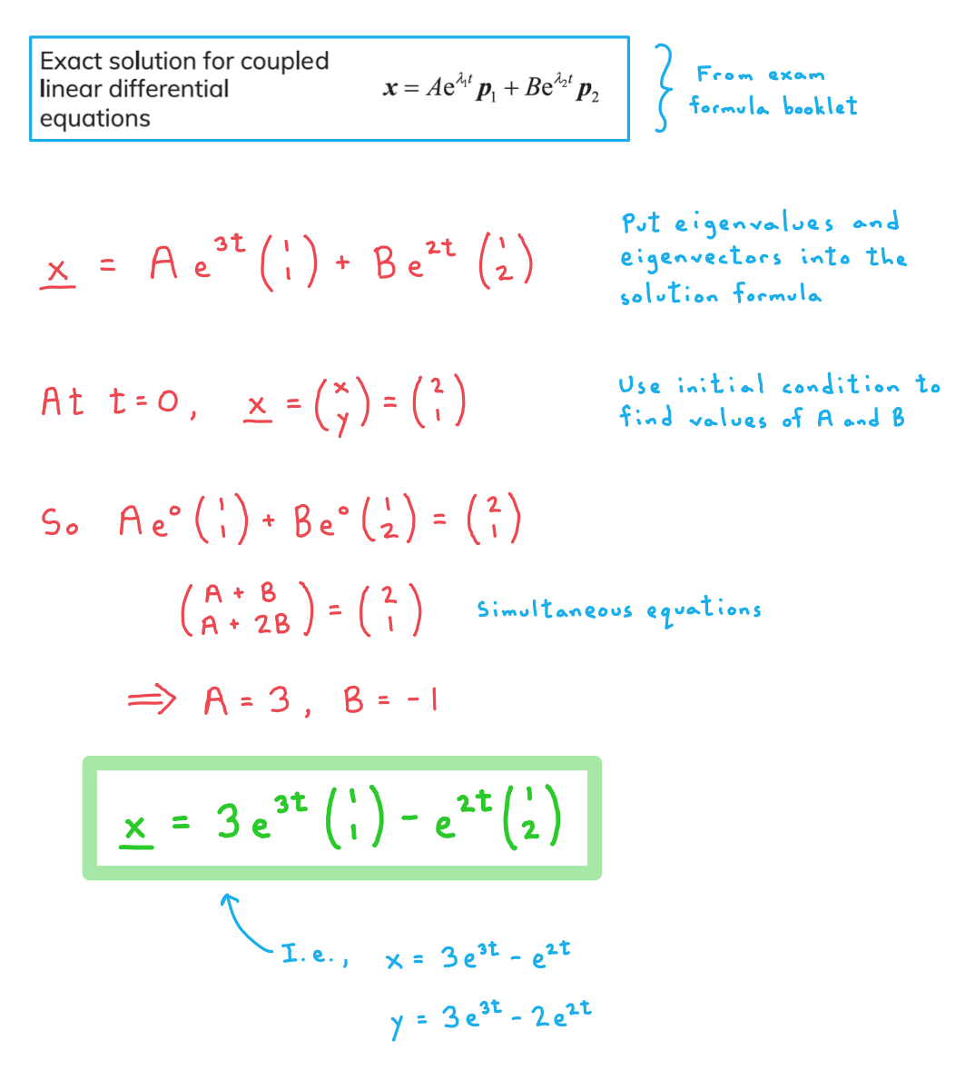
Phase Portraits
What is a phase portrait for a system of coupled differential equations?
- Here we are again considering systems of coupled equations that can be represented in the matrix form
format('truetype')%3Bfont-weight%3Anormal%3Bfont-style%3Anormal%3B%7D%3C%2Fstyle%3E%3C%2Fdefs%3E%3Ctext%20font-family%3D%22math1dd165a6c6b5bc8158c57065d13%22%20font-size%3D%2212%22%20font-weight%3D%22bold%22%20text-anchor%3D%22middle%22%20x%3D%225.5%22%20y%3D%226%22%3E.%3C%2Ftext%3E%3Ctext%20font-family%3D%22Times%20New%20Roman%22%20font-size%3D%2218%22%20font-style%3D%22italic%22%20font-weight%3D%22bold%22%20text-anchor%3D%22middle%22%20x%3D%225.5%22%20y%3D%2218%22%3Ex%3C%2Ftext%3E%3Ctext%20font-family%3D%22math1dd165a6c6b5bc8158c57065d13%22%20font-size%3D%2216%22%20text-anchor%3D%22middle%22%20x%3D%2219.5%22%20y%3D%2218%22%3E%3D%3C%2Ftext%3E%3Ctext%20font-family%3D%22Times%20New%20Roman%22%20font-size%3D%2218%22%20font-style%3D%22italic%22%20font-weight%3D%22bold%22%20text-anchor%3D%22middle%22%20x%3D%2236.5%22%20y%3D%2218%22%3EM%3C%2Ftext%3E%3Ctext%20font-family%3D%22Times%20New%20Roman%22%20font-size%3D%2218%22%20font-style%3D%22italic%22%20font-weight%3D%22bold%22%20text-anchor%3D%22middle%22%20x%3D%2250.5%22%20y%3D%2218%22%3Ex%3C%2Ftext%3E%3C%2Fsvg%3E) , where , , and
, where , , and - A phase portrait is a diagram showing how the values of x and y change over time
- On a phase portrait we will usually sketch several typical solution trajectories
- The precise trajectory that the solution for a particular system will travel along is determined by the initial conditions for the system
- Let and be the eigenvalues of the matrix
- The overall nature of the phase portrait depends in large part on the values of and
What does the phase portrait look like when and are real numbers?
- Recall that for real distinct eigenvalues the solution to a system of the above form is
format('truetype')%3Bfont-weight%3Anormal%3Bfont-style%3Anormal%3B%7D%3C%2Fstyle%3E%3C%2Fdefs%3E%3Ctext%20font-family%3D%22Times%20New%20Roman%22%20font-size%3D%2218%22%20font-style%3D%22italic%22%20font-weight%3D%22bold%22%20text-anchor%3D%22middle%22%20x%3D%225.5%22%20y%3D%2223%22%3Ex%3C%2Ftext%3E%3Ctext%20font-family%3D%22math1564b4c0e54101ac57a0cb68c16%22%20font-size%3D%2216%22%20text-anchor%3D%22middle%22%20x%3D%2219.5%22%20y%3D%2223%22%3E%3D%3C%2Ftext%3E%3Ctext%20font-family%3D%22Times%20New%20Roman%22%20font-size%3D%2218%22%20font-style%3D%22italic%22%20text-anchor%3D%22middle%22%20x%3D%2234.5%22%20y%3D%2223%22%3EA%3C%2Ftext%3E%3Ctext%20font-family%3D%22Times%20New%20Roman%22%20font-size%3D%2218%22%20text-anchor%3D%22middle%22%20x%3D%2246.5%22%20y%3D%2223%22%3Ee%3C%2Ftext%3E%3Ctext%20font-family%3D%22Times%20New%20Roman%22%20font-size%3D%2213%22%20font-style%3D%22italic%22%20text-anchor%3D%22middle%22%20x%3D%2253.5%22%20y%3D%2212%22%3E%26%23x3BB%3B%3C%2Ftext%3E%3Ctext%20font-family%3D%22Times%20New%20Roman%22%20font-size%3D%2211%22%20text-anchor%3D%22middle%22%20x%3D%2260.5%22%20y%3D%2218%22%3E1%3C%2Ftext%3E%3Ctext%20font-family%3D%22Times%20New%20Roman%22%20font-size%3D%2213%22%20font-style%3D%22italic%22%20text-anchor%3D%22middle%22%20x%3D%2265.5%22%20y%3D%2212%22%3Et%3C%2Ftext%3E%3Ctext%20font-family%3D%22Times%20New%20Roman%22%20font-size%3D%2218%22%20font-style%3D%22italic%22%20font-weight%3D%22bold%22%20text-anchor%3D%22middle%22%20x%3D%2273.5%22%20y%3D%2223%22%3Ep%3C%2Ftext%3E%3Ctext%20font-family%3D%22Times%20New%20Roman%22%20font-size%3D%2213%22%20text-anchor%3D%22middle%22%20x%3D%2282.5%22%20y%3D%2231%22%3E1%3C%2Ftext%3E%3Ctext%20font-family%3D%22math1564b4c0e54101ac57a0cb68c16%22%20font-size%3D%2216%22%20font-weight%3D%22bold%22%20text-anchor%3D%22middle%22%20x%3D%2295.5%22%20y%3D%2223%22%3E%2B%3C%2Ftext%3E%3Ctext%20font-family%3D%22Times%20New%20Roman%22%20font-size%3D%2218%22%20font-style%3D%22italic%22%20text-anchor%3D%22middle%22%20x%3D%22110.5%22%20y%3D%2223%22%3EB%3C%2Ftext%3E%3Ctext%20font-family%3D%22Times%20New%20Roman%22%20font-size%3D%2218%22%20text-anchor%3D%22middle%22%20x%3D%22121.5%22%20y%3D%2223%22%3Ee%3C%2Ftext%3E%3Ctext%20font-family%3D%22Times%20New%20Roman%22%20font-size%3D%2213%22%20font-style%3D%22italic%22%20text-anchor%3D%22middle%22%20x%3D%22128.5%22%20y%3D%2212%22%3E%26%23x3BB%3B%3C%2Ftext%3E%3Ctext%20font-family%3D%22Times%20New%20Roman%22%20font-size%3D%2211%22%20text-anchor%3D%22middle%22%20x%3D%22135.5%22%20y%3D%2218%22%3E2%3C%2Ftext%3E%3Ctext%20font-family%3D%22Times%20New%20Roman%22%20font-size%3D%2213%22%20font-style%3D%22italic%22%20text-anchor%3D%22middle%22%20x%3D%22140.5%22%20y%3D%2212%22%3Et%3C%2Ftext%3E%3Ctext%20font-family%3D%22Times%20New%20Roman%22%20font-size%3D%2218%22%20font-style%3D%22italic%22%20font-weight%3D%22bold%22%20text-anchor%3D%22middle%22%20x%3D%22148.5%22%20y%3D%2223%22%3Ep%3C%2Ftext%3E%3Ctext%20font-family%3D%22Times%20New%20Roman%22%20font-size%3D%2213%22%20font-weight%3D%22bold%22%20text-anchor%3D%22middle%22%20x%3D%22157.5%22%20y%3D%2231%22%3E2%3C%2Ftext%3E%3C%2Fsvg%3E) , where and are the eigenvalues of and and are the corresponding eigenvectors
, where and are the eigenvalues of and and are the corresponding eigenvectors
- AI HL only considers cases where and are distinct (i.e.,
format('truetype')%3Bfont-weight%3Anormal%3Bfont-style%3Anormal%3B%7D%3C%2Fstyle%3E%3C%2Fdefs%3E%3Ctext%20font-family%3D%22Times%20New%20Roman%22%20font-size%3D%2218%22%20font-style%3D%22italic%22%20text-anchor%3D%22middle%22%20x%3D%224.5%22%20y%3D%2216%22%3E%26%23x3BB%3B%3C%2Ftext%3E%3Ctext%20font-family%3D%22Times%20New%20Roman%22%20font-size%3D%2213%22%20text-anchor%3D%22middle%22%20x%3D%2213.5%22%20y%3D%2224%22%3E1%3C%2Ftext%3E%3Ctext%20font-family%3D%22math17ac52e3f2729d1b3f6d2b7e8f6%22%20font-size%3D%2216%22%20text-anchor%3D%22middle%22%20x%3D%2225.5%22%20y%3D%2216%22%3E%26%23x2260%3B%3C%2Ftext%3E%3Ctext%20font-family%3D%22Times%20New%20Roman%22%20font-size%3D%2218%22%20font-style%3D%22italic%22%20text-anchor%3D%22middle%22%20x%3D%2238.5%22%20y%3D%2216%22%3E%26%23x3BB%3B%3C%2Ftext%3E%3Ctext%20font-family%3D%22Times%20New%20Roman%22%20font-size%3D%2213%22%20text-anchor%3D%22middle%22%20x%3D%2247.5%22%20y%3D%2224%22%3E2%3C%2Ftext%3E%3C%2Fsvg%3E) ) and non-zero
) and non-zero
- AI HL only considers cases where
- A phase portrait will always include two ‘eigenvector lines’ through the origin, each one parallel to one of the eigenvectors
-
- So if
format('truetype')%3Bfont-weight%3Anormal%3Bfont-style%3Anormal%3B%7D%40font-face%7Bfont-family%3A'brack_sm2882ad605b1e27be87c7468'%3Bsrc%3Aurl(data%3Afont%2Ftruetype%3Bcharset%3Dutf-8%3Bbase64%2CAAEAAAAMAIAAAwBAT1MvMi7PH4UAAADMAAAATmNtYXA3kjw6AAABHAAAADxjdnQgAQYDiAAAAVgAAAASZ2x5ZkyYQ7YAAAFsAAAAkWhlYWQLyR8fAAACAAAAADZoaGVhAq0XCAAAAjgAAAAkaG10eDEjA%2FUAAAJcAAAADGxvY2EAAEKZAAACaAAAABBtYXhwBJsEcQAAAngAAAAgbmFtZW7QvZAAAAKYAAAB5XBvc3QArQBVAAAEgAAAACBwcmVwu5WEAAAABKAAAAAHAAACDAGQAAUAAAQABAAAAAAABAAEAAAAAAAAAQEAAAAAAAAAAAAAAAAAAAAAAAAAAAAAAAAAAAAAACAgICAAAAAg9AMD%2FP%2F8AAABVAABAAAAAAACAAEAAQAAABQAAwABAAAAFAAEACgAAAAGAAQAAQACI5wjn%2F%2F%2FAAAjnCOf%2F%2F%2FcZdxjAAEAAAAAAAAAAAFUAFQBAAArAIwAgACoAAcAAAACAAAAAADVAQEAAwAHAAAxMxEjFyM1M9XVq4CAAQHWqwABAAAAAABVAVgAAwAfGAGwAy%2BwADyxAgL1sAE8ALEDAD%2BwAjx8sQAG9bABPBEzESNVVQFY%2FqgAAQDXAAABLAFUAAMAIBgBsAUvsAE8sAI8sQAC9bADPACwAy%2BwAjyxAAH1sAE8EzMRI9dVVQFU%2FqwAAAAAAQAAAAEAAIsesexfDzz1AAMEAP%2F%2F%2F%2F%2FVre5k%2F%2F%2F%2F%2F9Wt7mT%2FgP%2F%2FAdYBWAAAAAoAAgABAAAAAAABAAABVP%2F%2FAAAXcP%2BA%2F4AB1gABAAAAAAAAAAAAAAAAAAAAAwDVAAABLAAAASwA1wAAAAAAAAAhAAAAWAAAAJEAAQAAAAMACgACAAAAAAACAIAEAAAAAAAEAABlAAAAAAAAABUBAgAAAAAAAAABACYAAAAAAAAAAAACAA4AJgAAAAAAAAADAEQANAAAAAAAAAAEACYAeAAAAAAAAAAFABYAngAAAAAAAAAGABMAtAAAAAAAAAAIABwAxwABAAAAAAABACYAAAABAAAAAAACAA4AJgABAAAAAAADAEQANAABAAAAAAAEACYAeAABAAAAAAAFABYAngABAAAAAAAGABMAtAABAAAAAAAIABwAxwADAAEECQABACYAAAADAAEECQACAA4AJgADAAEECQADAEQANAADAAEECQAEACYAeAADAAEECQAFABYAngADAAEECQAGABMAtAADAAEECQAIABwAxwBCAHIAYQBjAGsAZQB0AHMAIABzAG0AYQBsAGwAIABzAGkAegBlAFIAZQBnAHUAbABhAHIATQBhAHQAaABzACAARgBvAHIAIABNAG8AcgBlACAAQgByAGEAYwBrAGUAdABzACAAcwBtAGEAbABsACAAcwBpAHoAZQBCAHIAYQBjAGsAZQB0AHMAIABzAG0AYQBsAGwAIABzAGkAegBlAFYAZQByAHMAaQBvAG4AIAAyAC4AMEJyYWNrZXRzX3NtYWxsX3NpemUATQBhAHQAaABzACAARgBvAHIAIABNAG8AcgBlAAAAAAMAAAAAAAAAqgBVAAAAAAAAAAAAAAAAAAAAAAAAAAC5B%2F8AAo2FAA%3D%3D)format('truetype')%3Bfont-weight%3Anormal%3Bfont-style%3Anormal%3B%7D%40font-face%7Bfont-family%3A'bracketse552f5417ff4680c6b50499'%3Bsrc%3Aurl(data%3Afont%2Ftruetype%3Bcharset%3Dutf-8%3Bbase64%2CAAEAAAAMAIAAAwBAT1MvMi7RIisAAADMAAAATmNtYXBi7uzYAAABHAAAAExjdnQgBAkDLgAAAWgAAAASZ2x5Zo64f%2BkAAAF8AAABSWhlYWQLniGcAAACyAAAADZoaGVhBK4XLAAAAwAAAAAkaG10eCWq%2F90AAAMkAAAAFGxvY2EAABknAAADOAAAABhtYXhwBJIESAAAA1AAAAAgbmFtZRAA8I4AAANwAAAB3nBvc3QBwwDgAAAFUAAAACBwcmVwupWEAAAABXAAAAAHAAACggGQAAUAAAQABAAAAAAABAAEAAAAAAAAAQEAAAAAAAAAAAAAAAAAAAAAAAAAAAAAAAAAAAAAACAgICAAAAAg9AMEAAAAAAADgAAAAAAAAAACAAEAAQAAABQAAwABAAAAFAAEADgAAAAKAAgAAgACI5sjnSOeI6D%2F%2FwAAI5sjnSOeI6D%2F%2F9xm3GXcZdxkAAEAAAAAAAAAAAAAAAABVABWAQAALACoA4AAMgAHAAAAAgAAACoA1QNVAAMABwAANTMRIxMjETPV1auAgCoDK%2F0AAtUAAQAAAAABgAOAAAUAJBgBsAAvsAPFsQEC%2FbADELEEBP0AsQAAP7ABPLEEBj%2BwAzwwMTEzEAEjAFUBKyv%2BqwH8AYT%2BqgABAAAAAAGAA4AABQAmGAGwAC6wA8WxBQL9sAMQsQIE%2FQB8sQAGPxiwBTyxAwb2sAI8MDEREgEzABMBAVQr%2FtMCA4D91v6qAYQB%2FAAB%2F6wAAAEsA4AABQAnGAGwAC%2BwBzywA8WxAQL9sAMQsQQE%2FQCxAAA%2FsAE8sQQGP7ADPDAxISMSATMAASxVAf7UKwFVAfwBhP6rAAH%2FrAAAASwDgAAFACkYAbABL7AHPLAExbEAAv2wBBCxAwT9AHyxAQY%2FsAA8GLEEAD%2BwAzwwMRMzEAEjANdV%2FqsrASsDgP3V%2FqsBhgAAAAABAAAAAQAAeuTcpl8PPPUAAwQA%2F%2F%2F%2F%2F9Wt7o7%2F%2F%2F%2F%2F1a3ujv%2BsAAABgAOAAAAACgACAAEAAAAAAAEAAAOAAAAAABdw%2F6z%2FrAGAAAEAAAAAAAAAAAAAAAAAAAAFANUAAAEsAAABLAAAASz%2FrAEs%2F6wAAAAAAAAAJAAAAGgAAACzAAAA%2FQAAAUkAAQAAAAUACAACAAAAAAACAIAEAAAAAAAEAAA%2BAAAAAAAAABUBAgAAAAAAAAABACQAAAAAAAAAAAACAA4AJAAAAAAAAAADAEIAMgAAAAAAAAAEACQAdAAAAAAAAAAFABYAmAAAAAAAAAAGABIArgAAAAAAAAAIABwAwAABAAAAAAABACQAAAABAAAAAAACAA4AJAABAAAAAAADAEIAMgABAAAAAAAEACQAdAABAAAAAAAFABYAmAABAAAAAAAGABIArgABAAAAAAAIABwAwAADAAEECQABACQAAAADAAEECQACAA4AJAADAAEECQADAEIAMgADAAEECQAEACQAdAADAAEECQAFABYAmAADAAEECQAGABIArgADAAEECQAIABwAwABCAHIAYQBjAGsAZQB0AHMAIABmAHUAbABsACAAcwBpAHoAZQBSAGUAZwB1AGwAYQByAE0AYQB0AGgAcwAgAEYAbwByACAATQBvAHIAZQAgAEIAcgBhAGMAawBlAHQAcwAgAGYAdQBsAGwAIABzAGkAegBlAEIAcgBhAGMAawBlAHQAcwAgAGYAdQBsAGwAIABzAGkAegBlAFYAZQByAHMAaQBvAG4AIAAyAC4AMEJyYWNrZXRzX2Z1bGxfc2l6ZQBNAGEAdABoAHMAIABGAG8AcgAgAE0AbwByAGUAAAADAAAAAAAAAcAA4AAAAAAAAAAAAAAAAAAAAAAAAAAAuQf%2FAAGNhQA%3D)format('truetype')%3Bfont-weight%3Anormal%3Bfont-style%3Anormal%3B%7D%3C%2Fstyle%3E%3C%2Fdefs%3E%3Ctext%20font-family%3D%22Times%20New%20Roman%22%20font-size%3D%2218%22%20font-style%3D%22italic%22%20font-weight%3D%22bold%22%20text-anchor%3D%22middle%22%20x%3D%225.5%22%20y%3D%2233%22%3Ep%3C%2Ftext%3E%3Ctext%20font-family%3D%22Times%20New%20Roman%22%20font-size%3D%2213%22%20text-anchor%3D%22middle%22%20x%3D%2214.5%22%20y%3D%2241%22%3E1%3C%2Ftext%3E%3Ctext%20font-family%3D%22math17f39f8317fbdb1988ef4c628eb%22%20font-size%3D%2216%22%20text-anchor%3D%22middle%22%20x%3D%2226.5%22%20y%3D%2233%22%3E%3D%3C%2Ftext%3E%3Ctext%20font-family%3D%22bracketse552f5417ff4680c6b50499%22%20font-size%3D%2218%22%20text-anchor%3D%22start%22%20x%3D%2236.5%22%20y%3D%2218%22%3E%26%23x239B%3B%3C%2Ftext%3E%3Ctext%20font-family%3D%22brack_sm2882ad605b1e27be87c7468%22%20font-size%3D%2218%22%20text-anchor%3D%22start%22%20x%3D%2236.5%22%20y%3D%2224%22%3E%26%23x239C%3B%3C%2Ftext%3E%3Ctext%20font-family%3D%22brack_sm2882ad605b1e27be87c7468%22%20font-size%3D%2218%22%20text-anchor%3D%22start%22%20x%3D%2236.5%22%20y%3D%2230%22%3E%26%23x239C%3B%3C%2Ftext%3E%3Ctext%20font-family%3D%22brack_sm2882ad605b1e27be87c7468%22%20font-size%3D%2218%22%20text-anchor%3D%22start%22%20x%3D%2236.5%22%20y%3D%2236%22%3E%26%23x239C%3B%3C%2Ftext%3E%3Ctext%20font-family%3D%22bracketse552f5417ff4680c6b50499%22%20font-size%3D%2218%22%20text-anchor%3D%22start%22%20x%3D%2236.5%22%20y%3D%2252%22%3E%26%23x239D%3B%3C%2Ftext%3E%3Ctext%20font-family%3D%22bracketse552f5417ff4680c6b50499%22%20font-size%3D%2218%22%20text-anchor%3D%22start%22%20x%3D%2260.5%22%20y%3D%2218%22%3E%26%23x239E%3B%3C%2Ftext%3E%3Ctext%20font-family%3D%22brack_sm2882ad605b1e27be87c7468%22%20font-size%3D%2218%22%20text-anchor%3D%22start%22%20x%3D%2260.5%22%20y%3D%2224%22%3E%26%23x239F%3B%3C%2Ftext%3E%3Ctext%20font-family%3D%22brack_sm2882ad605b1e27be87c7468%22%20font-size%3D%2218%22%20text-anchor%3D%22start%22%20x%3D%2260.5%22%20y%3D%2230%22%3E%26%23x239F%3B%3C%2Ftext%3E%3Ctext%20font-family%3D%22brack_sm2882ad605b1e27be87c7468%22%20font-size%3D%2218%22%20text-anchor%3D%22start%22%20x%3D%2260.5%22%20y%3D%2236%22%3E%26%23x239F%3B%3C%2Ftext%3E%3Ctext%20font-family%3D%22bracketse552f5417ff4680c6b50499%22%20font-size%3D%2218%22%20text-anchor%3D%22start%22%20x%3D%2260.5%22%20y%3D%2252%22%3E%26%23x23A0%3B%3C%2Ftext%3E%3Ctext%20font-family%3D%22Times%20New%20Roman%22%20font-size%3D%2218%22%20text-anchor%3D%22middle%22%20x%3D%2250.5%22%20y%3D%2219%22%3E1%3C%2Ftext%3E%3Ctext%20font-family%3D%22Times%20New%20Roman%22%20font-size%3D%2218%22%20text-anchor%3D%22middle%22%20x%3D%2250.5%22%20y%3D%2245%22%3E2%3C%2Ftext%3E%3C%2Fsvg%3E) and
and format('truetype')%3Bfont-weight%3Anormal%3Bfont-style%3Anormal%3B%7D%40font-face%7Bfont-family%3A'brack_sm2882ad605b1e27be87c7468'%3Bsrc%3Aurl(data%3Afont%2Ftruetype%3Bcharset%3Dutf-8%3Bbase64%2CAAEAAAAMAIAAAwBAT1MvMi7PH4UAAADMAAAATmNtYXA3kjw6AAABHAAAADxjdnQgAQYDiAAAAVgAAAASZ2x5ZkyYQ7YAAAFsAAAAkWhlYWQLyR8fAAACAAAAADZoaGVhAq0XCAAAAjgAAAAkaG10eDEjA%2FUAAAJcAAAADGxvY2EAAEKZAAACaAAAABBtYXhwBJsEcQAAAngAAAAgbmFtZW7QvZAAAAKYAAAB5XBvc3QArQBVAAAEgAAAACBwcmVwu5WEAAAABKAAAAAHAAACDAGQAAUAAAQABAAAAAAABAAEAAAAAAAAAQEAAAAAAAAAAAAAAAAAAAAAAAAAAAAAAAAAAAAAACAgICAAAAAg9AMD%2FP%2F8AAABVAABAAAAAAACAAEAAQAAABQAAwABAAAAFAAEACgAAAAGAAQAAQACI5wjn%2F%2F%2FAAAjnCOf%2F%2F%2FcZdxjAAEAAAAAAAAAAAFUAFQBAAArAIwAgACoAAcAAAACAAAAAADVAQEAAwAHAAAxMxEjFyM1M9XVq4CAAQHWqwABAAAAAABVAVgAAwAfGAGwAy%2BwADyxAgL1sAE8ALEDAD%2BwAjx8sQAG9bABPBEzESNVVQFY%2FqgAAQDXAAABLAFUAAMAIBgBsAUvsAE8sAI8sQAC9bADPACwAy%2BwAjyxAAH1sAE8EzMRI9dVVQFU%2FqwAAAAAAQAAAAEAAIsesexfDzz1AAMEAP%2F%2F%2F%2F%2FVre5k%2F%2F%2F%2F%2F9Wt7mT%2FgP%2F%2FAdYBWAAAAAoAAgABAAAAAAABAAABVP%2F%2FAAAXcP%2BA%2F4AB1gABAAAAAAAAAAAAAAAAAAAAAwDVAAABLAAAASwA1wAAAAAAAAAhAAAAWAAAAJEAAQAAAAMACgACAAAAAAACAIAEAAAAAAAEAABlAAAAAAAAABUBAgAAAAAAAAABACYAAAAAAAAAAAACAA4AJgAAAAAAAAADAEQANAAAAAAAAAAEACYAeAAAAAAAAAAFABYAngAAAAAAAAAGABMAtAAAAAAAAAAIABwAxwABAAAAAAABACYAAAABAAAAAAACAA4AJgABAAAAAAADAEQANAABAAAAAAAEACYAeAABAAAAAAAFABYAngABAAAAAAAGABMAtAABAAAAAAAIABwAxwADAAEECQABACYAAAADAAEECQACAA4AJgADAAEECQADAEQANAADAAEECQAEACYAeAADAAEECQAFABYAngADAAEECQAGABMAtAADAAEECQAIABwAxwBCAHIAYQBjAGsAZQB0AHMAIABzAG0AYQBsAGwAIABzAGkAegBlAFIAZQBnAHUAbABhAHIATQBhAHQAaABzACAARgBvAHIAIABNAG8AcgBlACAAQgByAGEAYwBrAGUAdABzACAAcwBtAGEAbABsACAAcwBpAHoAZQBCAHIAYQBjAGsAZQB0AHMAIABzAG0AYQBsAGwAIABzAGkAegBlAFYAZQByAHMAaQBvAG4AIAAyAC4AMEJyYWNrZXRzX3NtYWxsX3NpemUATQBhAHQAaABzACAARgBvAHIAIABNAG8AcgBlAAAAAAMAAAAAAAAAqgBVAAAAAAAAAAAAAAAAAAAAAAAAAAC5B%2F8AAo2FAA%3D%3D)format('truetype')%3Bfont-weight%3Anormal%3Bfont-style%3Anormal%3B%7D%40font-face%7Bfont-family%3A'bracketse552f5417ff4680c6b50499'%3Bsrc%3Aurl(data%3Afont%2Ftruetype%3Bcharset%3Dutf-8%3Bbase64%2CAAEAAAAMAIAAAwBAT1MvMi7RIisAAADMAAAATmNtYXBi7uzYAAABHAAAAExjdnQgBAkDLgAAAWgAAAASZ2x5Zo64f%2BkAAAF8AAABSWhlYWQLniGcAAACyAAAADZoaGVhBK4XLAAAAwAAAAAkaG10eCWq%2F90AAAMkAAAAFGxvY2EAABknAAADOAAAABhtYXhwBJIESAAAA1AAAAAgbmFtZRAA8I4AAANwAAAB3nBvc3QBwwDgAAAFUAAAACBwcmVwupWEAAAABXAAAAAHAAACggGQAAUAAAQABAAAAAAABAAEAAAAAAAAAQEAAAAAAAAAAAAAAAAAAAAAAAAAAAAAAAAAAAAAACAgICAAAAAg9AMEAAAAAAADgAAAAAAAAAACAAEAAQAAABQAAwABAAAAFAAEADgAAAAKAAgAAgACI5sjnSOeI6D%2F%2FwAAI5sjnSOeI6D%2F%2F9xm3GXcZdxkAAEAAAAAAAAAAAAAAAABVABWAQAALACoA4AAMgAHAAAAAgAAACoA1QNVAAMABwAANTMRIxMjETPV1auAgCoDK%2F0AAtUAAQAAAAABgAOAAAUAJBgBsAAvsAPFsQEC%2FbADELEEBP0AsQAAP7ABPLEEBj%2BwAzwwMTEzEAEjAFUBKyv%2BqwH8AYT%2BqgABAAAAAAGAA4AABQAmGAGwAC6wA8WxBQL9sAMQsQIE%2FQB8sQAGPxiwBTyxAwb2sAI8MDEREgEzABMBAVQr%2FtMCA4D91v6qAYQB%2FAAB%2F6wAAAEsA4AABQAnGAGwAC%2BwBzywA8WxAQL9sAMQsQQE%2FQCxAAA%2FsAE8sQQGP7ADPDAxISMSATMAASxVAf7UKwFVAfwBhP6rAAH%2FrAAAASwDgAAFACkYAbABL7AHPLAExbEAAv2wBBCxAwT9AHyxAQY%2FsAA8GLEEAD%2BwAzwwMRMzEAEjANdV%2FqsrASsDgP3V%2FqsBhgAAAAABAAAAAQAAeuTcpl8PPPUAAwQA%2F%2F%2F%2F%2F9Wt7o7%2F%2F%2F%2F%2F1a3ujv%2BsAAABgAOAAAAACgACAAEAAAAAAAEAAAOAAAAAABdw%2F6z%2FrAGAAAEAAAAAAAAAAAAAAAAAAAAFANUAAAEsAAABLAAAASz%2FrAEs%2F6wAAAAAAAAAJAAAAGgAAACzAAAA%2FQAAAUkAAQAAAAUACAACAAAAAAACAIAEAAAAAAAEAAA%2BAAAAAAAAABUBAgAAAAAAAAABACQAAAAAAAAAAAACAA4AJAAAAAAAAAADAEIAMgAAAAAAAAAEACQAdAAAAAAAAAAFABYAmAAAAAAAAAAGABIArgAAAAAAAAAIABwAwAABAAAAAAABACQAAAABAAAAAAACAA4AJAABAAAAAAADAEIAMgABAAAAAAAEACQAdAABAAAAAAAFABYAmAABAAAAAAAGABIArgABAAAAAAAIABwAwAADAAEECQABACQAAAADAAEECQACAA4AJAADAAEECQADAEIAMgADAAEECQAEACQAdAADAAEECQAFABYAmAADAAEECQAGABIArgADAAEECQAIABwAwABCAHIAYQBjAGsAZQB0AHMAIABmAHUAbABsACAAcwBpAHoAZQBSAGUAZwB1AGwAYQByAE0AYQB0AGgAcwAgAEYAbwByACAATQBvAHIAZQAgAEIAcgBhAGMAawBlAHQAcwAgAGYAdQBsAGwAIABzAGkAegBlAEIAcgBhAGMAawBlAHQAcwAgAGYAdQBsAGwAIABzAGkAegBlAFYAZQByAHMAaQBvAG4AIAAyAC4AMEJyYWNrZXRzX2Z1bGxfc2l6ZQBNAGEAdABoAHMAIABGAG8AcgAgAE0AbwByAGUAAAADAAAAAAAAAcAA4AAAAAAAAAAAAAAAAAAAAAAAAAAAuQf%2FAAGNhQA%3D)format('truetype')%3Bfont-weight%3Anormal%3Bfont-style%3Anormal%3B%7D%3C%2Fstyle%3E%3C%2Fdefs%3E%3Ctext%20font-family%3D%22Times%20New%20Roman%22%20font-size%3D%2218%22%20font-style%3D%22italic%22%20font-weight%3D%22bold%22%20text-anchor%3D%22middle%22%20x%3D%225.5%22%20y%3D%2233%22%3Ep%3C%2Ftext%3E%3Ctext%20font-family%3D%22Times%20New%20Roman%22%20font-size%3D%2213%22%20text-anchor%3D%22middle%22%20x%3D%2214.5%22%20y%3D%2241%22%3E2%3C%2Ftext%3E%3Ctext%20font-family%3D%22math143f4d31b04031e49f5eb18baba%22%20font-size%3D%2216%22%20text-anchor%3D%22middle%22%20x%3D%2226.5%22%20y%3D%2233%22%3E%3D%3C%2Ftext%3E%3Ctext%20font-family%3D%22bracketse552f5417ff4680c6b50499%22%20font-size%3D%2218%22%20text-anchor%3D%22start%22%20x%3D%2236.5%22%20y%3D%2218%22%3E%26%23x239B%3B%3C%2Ftext%3E%3Ctext%20font-family%3D%22brack_sm2882ad605b1e27be87c7468%22%20font-size%3D%2218%22%20text-anchor%3D%22start%22%20x%3D%2236.5%22%20y%3D%2224%22%3E%26%23x239C%3B%3C%2Ftext%3E%3Ctext%20font-family%3D%22brack_sm2882ad605b1e27be87c7468%22%20font-size%3D%2218%22%20text-anchor%3D%22start%22%20x%3D%2236.5%22%20y%3D%2230%22%3E%26%23x239C%3B%3C%2Ftext%3E%3Ctext%20font-family%3D%22brack_sm2882ad605b1e27be87c7468%22%20font-size%3D%2218%22%20text-anchor%3D%22start%22%20x%3D%2236.5%22%20y%3D%2236%22%3E%26%23x239C%3B%3C%2Ftext%3E%3Ctext%20font-family%3D%22bracketse552f5417ff4680c6b50499%22%20font-size%3D%2218%22%20text-anchor%3D%22start%22%20x%3D%2236.5%22%20y%3D%2252%22%3E%26%23x239D%3B%3C%2Ftext%3E%3Ctext%20font-family%3D%22bracketse552f5417ff4680c6b50499%22%20font-size%3D%2218%22%20text-anchor%3D%22start%22%20x%3D%2273.5%22%20y%3D%2218%22%3E%26%23x239E%3B%3C%2Ftext%3E%3Ctext%20font-family%3D%22brack_sm2882ad605b1e27be87c7468%22%20font-size%3D%2218%22%20text-anchor%3D%22start%22%20x%3D%2273.5%22%20y%3D%2224%22%3E%26%23x239F%3B%3C%2Ftext%3E%3Ctext%20font-family%3D%22brack_sm2882ad605b1e27be87c7468%22%20font-size%3D%2218%22%20text-anchor%3D%22start%22%20x%3D%2273.5%22%20y%3D%2230%22%3E%26%23x239F%3B%3C%2Ftext%3E%3Ctext%20font-family%3D%22brack_sm2882ad605b1e27be87c7468%22%20font-size%3D%2218%22%20text-anchor%3D%22start%22%20x%3D%2273.5%22%20y%3D%2236%22%3E%26%23x239F%3B%3C%2Ftext%3E%3Ctext%20font-family%3D%22bracketse552f5417ff4680c6b50499%22%20font-size%3D%2218%22%20text-anchor%3D%22start%22%20x%3D%2273.5%22%20y%3D%2252%22%3E%26%23x23A0%3B%3C%2Ftext%3E%3Ctext%20font-family%3D%22math143f4d31b04031e49f5eb18baba%22%20font-size%3D%2216%22%20text-anchor%3D%22middle%22%20x%3D%2252.5%22%20y%3D%2219%22%3E%26%23x2212%3B%3C%2Ftext%3E%3Ctext%20font-family%3D%22Times%20New%20Roman%22%20font-size%3D%2218%22%20text-anchor%3D%22middle%22%20x%3D%2263.5%22%20y%3D%2219%22%3E3%3C%2Ftext%3E%3Ctext%20font-family%3D%22Times%20New%20Roman%22%20font-size%3D%2218%22%20text-anchor%3D%22middle%22%20x%3D%2256.5%22%20y%3D%2245%22%3E4%3C%2Ftext%3E%3C%2Fsvg%3E) , for example, then these lines through the origin will have equations
, for example, then these lines through the origin will have equations format('truetype')%3Bfont-weight%3Anormal%3Bfont-style%3Anormal%3B%7D%3C%2Fstyle%3E%3C%2Fdefs%3E%3Ctext%20font-family%3D%22Times%20New%20Roman%22%20font-size%3D%2218%22%20font-style%3D%22italic%22%20text-anchor%3D%22middle%22%20x%3D%224.5%22%20y%3D%2216%22%3Ey%3C%2Ftext%3E%3Ctext%20font-family%3D%22math17f39f8317fbdb1988ef4c628eb%22%20font-size%3D%2216%22%20text-anchor%3D%22middle%22%20x%3D%2218.5%22%20y%3D%2216%22%3E%3D%3C%2Ftext%3E%3Ctext%20font-family%3D%22Times%20New%20Roman%22%20font-size%3D%2218%22%20text-anchor%3D%22middle%22%20x%3D%2231.5%22%20y%3D%2216%22%3E2%3C%2Ftext%3E%3Ctext%20font-family%3D%22Times%20New%20Roman%22%20font-size%3D%2218%22%20font-style%3D%22italic%22%20text-anchor%3D%22middle%22%20x%3D%2240.5%22%20y%3D%2216%22%3Ex%3C%2Ftext%3E%3C%2Fsvg%3E) and
and format('truetype')%3Bfont-weight%3Anormal%3Bfont-style%3Anormal%3B%7D%3C%2Fstyle%3E%3C%2Fdefs%3E%3Ctext%20font-family%3D%22Times%20New%20Roman%22%20font-size%3D%2218%22%20font-style%3D%22italic%22%20text-anchor%3D%22middle%22%20x%3D%224.5%22%20y%3D%2230%22%3Ey%3C%2Ftext%3E%3Ctext%20font-family%3D%22math143f4d31b04031e49f5eb18baba%22%20font-size%3D%2216%22%20text-anchor%3D%22middle%22%20x%3D%2218.5%22%20y%3D%2230%22%3E%3D%3C%2Ftext%3E%3Ctext%20font-family%3D%22math143f4d31b04031e49f5eb18baba%22%20font-size%3D%2216%22%20text-anchor%3D%22middle%22%20x%3D%2235.5%22%20y%3D%2230%22%3E%26%23x2212%3B%3C%2Ftext%3E%3Cline%20stroke%3D%22%23000000%22%20stroke-linecap%3D%22square%22%20stroke-width%3D%221%22%20x1%3D%2246.5%22%20x2%3D%2258.5%22%20y1%3D%2223.5%22%20y2%3D%2223.5%22%2F%3E%3Ctext%20font-family%3D%22Times%20New%20Roman%22%20font-size%3D%2218%22%20text-anchor%3D%22middle%22%20x%3D%2252.5%22%20y%3D%2216%22%3E4%3C%2Ftext%3E%3Ctext%20font-family%3D%22Times%20New%20Roman%22%20font-size%3D%2218%22%20text-anchor%3D%22middle%22%20x%3D%2252.5%22%20y%3D%2241%22%3E3%3C%2Ftext%3E%3Ctext%20font-family%3D%22Times%20New%20Roman%22%20font-size%3D%2218%22%20font-style%3D%22italic%22%20text-anchor%3D%22middle%22%20x%3D%2265.5%22%20y%3D%2230%22%3Ex%3C%2Ftext%3E%3C%2Fsvg%3E) , respectively
, respectively
- So if
- These lines will define two sets of solution trajectories
- If the eigenvalue corresponding to a line’s eigenvector is positive, then there will be solution trajectories along the line away from the origin in both directions as t increases
- If the eigenvalue corresponding to a line’s eigenvector is negative, then there will be solution trajectories along the line towards the origin in both directions as t increases
- No solution trajectory will ever cross an eigenvector line
-
- If both eigenvalues are positive then all solution trajectories will be directed away from the origin as t increases
- In between the ‘eigenvector lines’ the trajectories as they move away from the origin will all curve to become approximately parallel to the line whose eigenvector corresponds to the larger eigenvalue
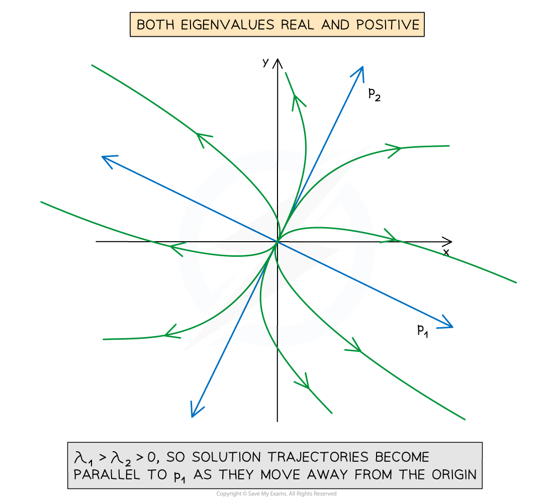
- If both eigenvalues are negative then all solution trajectories will be directed towards the origin as t increases
- In between the ‘eigenvector lines’ the trajectories will all curve so that at points further away from the origin they are approximately parallel to the line whose eigenvector corresponds to the more negative eigenvalue
- They will then converge on the other eigenvalue line as they move in towards the origin
- In between the ‘eigenvector lines’ the trajectories will all curve so that at points further away from the origin they are approximately parallel to the line whose eigenvector corresponds to the more negative eigenvalue
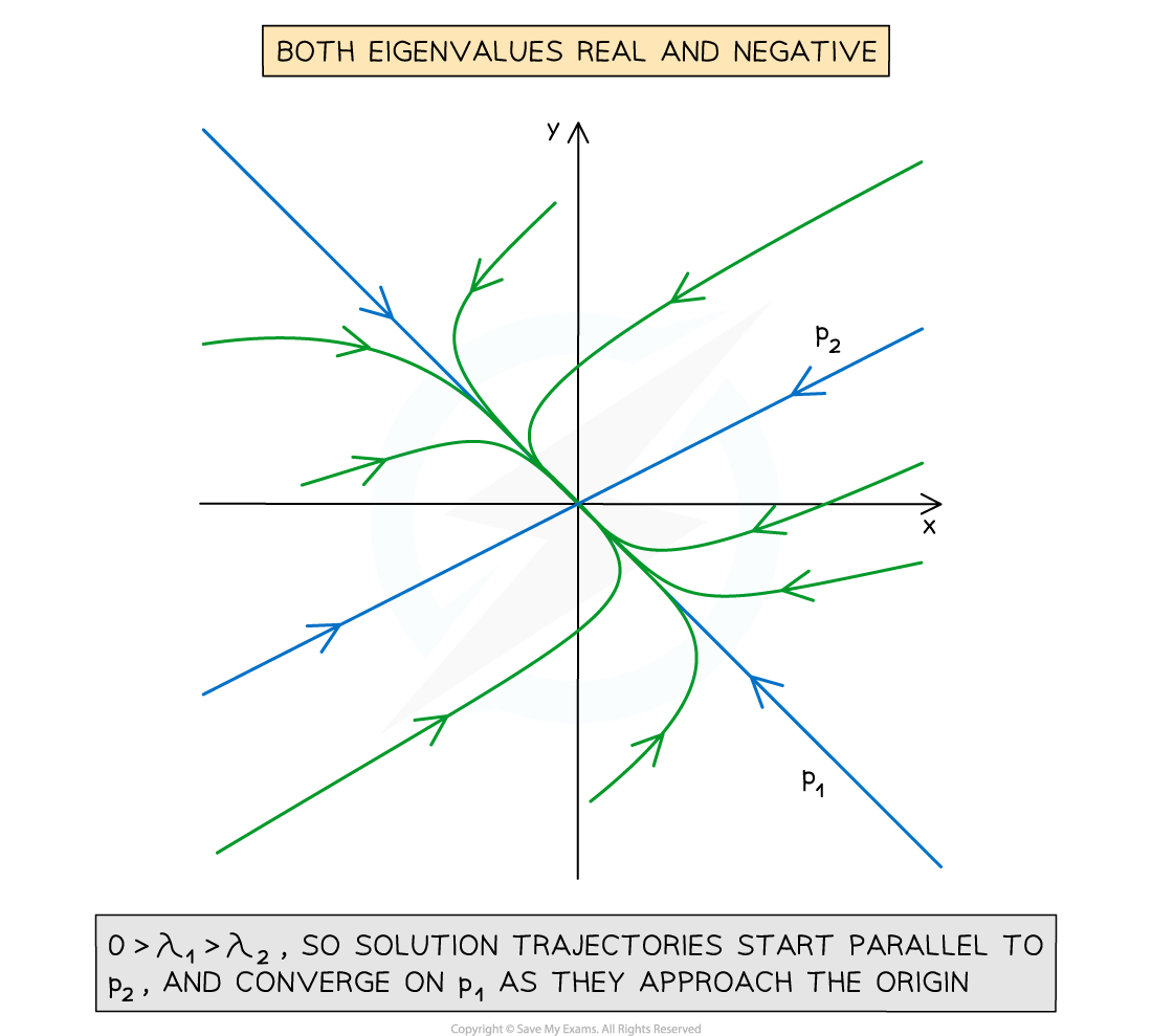
- If one eigenvalue is positive and one eigenvalue is negative then solution trajectories will generally start by heading in towards the origin before curving to head out away again from the origin as t increases
- In between the ‘eigenvector lines’ the solution trajectories will all move in towards the origin along the direction of the eigenvector line that corresponds to the negative eigenvalue, before curving away and converging on the eigenvector line that corresponds to the positive eigenvalue as they head away from the origin
What does the phase portrait look like when and are imaginary numbers?
- Here the solution trajectories will all be either circles or ellipses with their centres at the origin
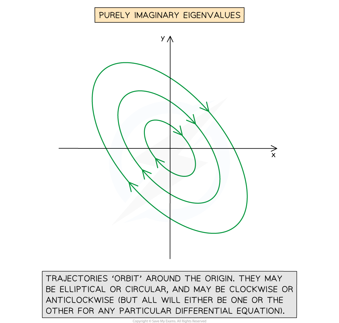
- You can determine the direction (clockwise or anticlockwise) and the shape (circular or elliptical) of the trajectories by considering the values of
 and
and  for points on the coordinate axes
 - For example, consider the system
format('truetype')%3Bfont-weight%3Anormal%3Bfont-style%3Anormal%3B%7D%40font-face%7Bfont-family%3A'brack_sm2882ad605b1e27be87c7468'%3Bsrc%3Aurl(data%3Afont%2Ftruetype%3Bcharset%3Dutf-8%3Bbase64%2CAAEAAAAMAIAAAwBAT1MvMi7PH4UAAADMAAAATmNtYXA3kjw6AAABHAAAADxjdnQgAQYDiAAAAVgAAAASZ2x5ZkyYQ7YAAAFsAAAAkWhlYWQLyR8fAAACAAAAADZoaGVhAq0XCAAAAjgAAAAkaG10eDEjA%2FUAAAJcAAAADGxvY2EAAEKZAAACaAAAABBtYXhwBJsEcQAAAngAAAAgbmFtZW7QvZAAAAKYAAAB5XBvc3QArQBVAAAEgAAAACBwcmVwu5WEAAAABKAAAAAHAAACDAGQAAUAAAQABAAAAAAABAAEAAAAAAAAAQEAAAAAAAAAAAAAAAAAAAAAAAAAAAAAAAAAAAAAACAgICAAAAAg9AMD%2FP%2F8AAABVAABAAAAAAACAAEAAQAAABQAAwABAAAAFAAEACgAAAAGAAQAAQACI5wjn%2F%2F%2FAAAjnCOf%2F%2F%2FcZdxjAAEAAAAAAAAAAAFUAFQBAAArAIwAgACoAAcAAAACAAAAAADVAQEAAwAHAAAxMxEjFyM1M9XVq4CAAQHWqwABAAAAAABVAVgAAwAfGAGwAy%2BwADyxAgL1sAE8ALEDAD%2BwAjx8sQAG9bABPBEzESNVVQFY%2FqgAAQDXAAABLAFUAAMAIBgBsAUvsAE8sAI8sQAC9bADPACwAy%2BwAjyxAAH1sAE8EzMRI9dVVQFU%2FqwAAAAAAQAAAAEAAIsesexfDzz1AAMEAP%2F%2F%2F%2F%2FVre5k%2F%2F%2F%2F%2F9Wt7mT%2FgP%2F%2FAdYBWAAAAAoAAgABAAAAAAABAAABVP%2F%2FAAAXcP%2BA%2F4AB1gABAAAAAAAAAAAAAAAAAAAAAwDVAAABLAAAASwA1wAAAAAAAAAhAAAAWAAAAJEAAQAAAAMACgACAAAAAAACAIAEAAAAAAAEAABlAAAAAAAAABUBAgAAAAAAAAABACYAAAAAAAAAAAACAA4AJgAAAAAAAAADAEQANAAAAAAAAAAEACYAeAAAAAAAAAAFABYAngAAAAAAAAAGABMAtAAAAAAAAAAIABwAxwABAAAAAAABACYAAAABAAAAAAACAA4AJgABAAAAAAADAEQANAABAAAAAAAEACYAeAABAAAAAAAFABYAngABAAAAAAAGABMAtAABAAAAAAAIABwAxwADAAEECQABACYAAAADAAEECQACAA4AJgADAAEECQADAEQANAADAAEECQAEACYAeAADAAEECQAFABYAngADAAEECQAGABMAtAADAAEECQAIABwAxwBCAHIAYQBjAGsAZQB0AHMAIABzAG0AYQBsAGwAIABzAGkAegBlAFIAZQBnAHUAbABhAHIATQBhAHQAaABzACAARgBvAHIAIABNAG8AcgBlACAAQgByAGEAYwBrAGUAdABzACAAcwBtAGEAbABsACAAcwBpAHoAZQBCAHIAYQBjAGsAZQB0AHMAIABzAG0AYQBsAGwAIABzAGkAegBlAFYAZQByAHMAaQBvAG4AIAAyAC4AMEJyYWNrZXRzX3NtYWxsX3NpemUATQBhAHQAaABzACAARgBvAHIAIABNAG8AcgBlAAAAAAMAAAAAAAAAqgBVAAAAAAAAAAAAAAAAAAAAAAAAAAC5B%2F8AAo2FAA%3D%3D)format('truetype')%3Bfont-weight%3Anormal%3Bfont-style%3Anormal%3B%7D%40font-face%7Bfont-family%3A'bracketse552f5417ff4680c6b50499'%3Bsrc%3Aurl(data%3Afont%2Ftruetype%3Bcharset%3Dutf-8%3Bbase64%2CAAEAAAAMAIAAAwBAT1MvMi7RIisAAADMAAAATmNtYXBi7uzYAAABHAAAAExjdnQgBAkDLgAAAWgAAAASZ2x5Zo64f%2BkAAAF8AAABSWhlYWQLniGcAAACyAAAADZoaGVhBK4XLAAAAwAAAAAkaG10eCWq%2F90AAAMkAAAAFGxvY2EAABknAAADOAAAABhtYXhwBJIESAAAA1AAAAAgbmFtZRAA8I4AAANwAAAB3nBvc3QBwwDgAAAFUAAAACBwcmVwupWEAAAABXAAAAAHAAACggGQAAUAAAQABAAAAAAABAAEAAAAAAAAAQEAAAAAAAAAAAAAAAAAAAAAAAAAAAAAAAAAAAAAACAgICAAAAAg9AMEAAAAAAADgAAAAAAAAAACAAEAAQAAABQAAwABAAAAFAAEADgAAAAKAAgAAgACI5sjnSOeI6D%2F%2FwAAI5sjnSOeI6D%2F%2F9xm3GXcZdxkAAEAAAAAAAAAAAAAAAABVABWAQAALACoA4AAMgAHAAAAAgAAACoA1QNVAAMABwAANTMRIxMjETPV1auAgCoDK%2F0AAtUAAQAAAAABgAOAAAUAJBgBsAAvsAPFsQEC%2FbADELEEBP0AsQAAP7ABPLEEBj%2BwAzwwMTEzEAEjAFUBKyv%2BqwH8AYT%2BqgABAAAAAAGAA4AABQAmGAGwAC6wA8WxBQL9sAMQsQIE%2FQB8sQAGPxiwBTyxAwb2sAI8MDEREgEzABMBAVQr%2FtMCA4D91v6qAYQB%2FAAB%2F6wAAAEsA4AABQAnGAGwAC%2BwBzywA8WxAQL9sAMQsQQE%2FQCxAAA%2FsAE8sQQGP7ADPDAxISMSATMAASxVAf7UKwFVAfwBhP6rAAH%2FrAAAASwDgAAFACkYAbABL7AHPLAExbEAAv2wBBCxAwT9AHyxAQY%2FsAA8GLEEAD%2BwAzwwMRMzEAEjANdV%2FqsrASsDgP3V%2FqsBhgAAAAABAAAAAQAAeuTcpl8PPPUAAwQA%2F%2F%2F%2F%2F9Wt7o7%2F%2F%2F%2F%2F1a3ujv%2BsAAABgAOAAAAACgACAAEAAAAAAAEAAAOAAAAAABdw%2F6z%2FrAGAAAEAAAAAAAAAAAAAAAAAAAAFANUAAAEsAAABLAAAASz%2FrAEs%2F6wAAAAAAAAAJAAAAGgAAACzAAAA%2FQAAAUkAAQAAAAUACAACAAAAAAACAIAEAAAAAAAEAAA%2BAAAAAAAAABUBAgAAAAAAAAABACQAAAAAAAAAAAACAA4AJAAAAAAAAAADAEIAMgAAAAAAAAAEACQAdAAAAAAAAAAFABYAmAAAAAAAAAAGABIArgAAAAAAAAAIABwAwAABAAAAAAABACQAAAABAAAAAAACAA4AJAABAAAAAAADAEIAMgABAAAAAAAEACQAdAABAAAAAAAFABYAmAABAAAAAAAGABIArgABAAAAAAAIABwAwAADAAEECQABACQAAAADAAEECQACAA4AJAADAAEECQADAEIAMgADAAEECQAEACQAdAADAAEECQAFABYAmAADAAEECQAGABIArgADAAEECQAIABwAwABCAHIAYQBjAGsAZQB0AHMAIABmAHUAbABsACAAcwBpAHoAZQBSAGUAZwB1AGwAYQByAE0AYQB0AGgAcwAgAEYAbwByACAATQBvAHIAZQAgAEIAcgBhAGMAawBlAHQAcwAgAGYAdQBsAGwAIABzAGkAegBlAEIAcgBhAGMAawBlAHQAcwAgAGYAdQBsAGwAIABzAGkAegBlAFYAZQByAHMAaQBvAG4AIAAyAC4AMEJyYWNrZXRzX2Z1bGxfc2l6ZQBNAGEAdABoAHMAIABGAG8AcgAgAE0AbwByAGUAAAADAAAAAAAAAcAA4AAAAAAAAAAAAAAAAAAAAAAAAAAAuQf%2FAAGNhQA%3D)format('truetype')%3Bfont-weight%3Anormal%3Bfont-style%3Anormal%3B%7D%3C%2Fstyle%3E%3C%2Fdefs%3E%3Ctext%20font-family%3D%22math16d8888858ea6f9ebce8ea398ff%22%20font-size%3D%2212%22%20font-weight%3D%22bold%22%20text-anchor%3D%22middle%22%20x%3D%225.5%22%20y%3D%2221%22%3E.%3C%2Ftext%3E%3Ctext%20font-family%3D%22Times%20New%20Roman%22%20font-size%3D%2218%22%20font-style%3D%22italic%22%20font-weight%3D%22bold%22%20text-anchor%3D%22middle%22%20x%3D%225.5%22%20y%3D%2233%22%3Ex%3C%2Ftext%3E%3Ctext%20font-family%3D%22math16d8888858ea6f9ebce8ea398ff%22%20font-size%3D%2216%22%20text-anchor%3D%22middle%22%20x%3D%2219.5%22%20y%3D%2233%22%3E%3D%3C%2Ftext%3E%3Ctext%20font-family%3D%22bracketse552f5417ff4680c6b50499%22%20font-size%3D%2218%22%20text-anchor%3D%22start%22%20x%3D%2229.5%22%20y%3D%2218%22%3E%26%23x239B%3B%3C%2Ftext%3E%3Ctext%20font-family%3D%22brack_sm2882ad605b1e27be87c7468%22%20font-size%3D%2218%22%20text-anchor%3D%22start%22%20x%3D%2229.5%22%20y%3D%2224%22%3E%26%23x239C%3B%3C%2Ftext%3E%3Ctext%20font-family%3D%22brack_sm2882ad605b1e27be87c7468%22%20font-size%3D%2218%22%20text-anchor%3D%22start%22%20x%3D%2229.5%22%20y%3D%2230%22%3E%26%23x239C%3B%3C%2Ftext%3E%3Ctext%20font-family%3D%22brack_sm2882ad605b1e27be87c7468%22%20font-size%3D%2218%22%20text-anchor%3D%22start%22%20x%3D%2229.5%22%20y%3D%2236%22%3E%26%23x239C%3B%3C%2Ftext%3E%3Ctext%20font-family%3D%22bracketse552f5417ff4680c6b50499%22%20font-size%3D%2218%22%20text-anchor%3D%22start%22%20x%3D%2229.5%22%20y%3D%2252%22%3E%26%23x239D%3B%3C%2Ftext%3E%3Ctext%20font-family%3D%22bracketse552f5417ff4680c6b50499%22%20font-size%3D%2218%22%20text-anchor%3D%22start%22%20x%3D%2283.5%22%20y%3D%2218%22%3E%26%23x239E%3B%3C%2Ftext%3E%3Ctext%20font-family%3D%22brack_sm2882ad605b1e27be87c7468%22%20font-size%3D%2218%22%20text-anchor%3D%22start%22%20x%3D%2283.5%22%20y%3D%2224%22%3E%26%23x239F%3B%3C%2Ftext%3E%3Ctext%20font-family%3D%22brack_sm2882ad605b1e27be87c7468%22%20font-size%3D%2218%22%20text-anchor%3D%22start%22%20x%3D%2283.5%22%20y%3D%2230%22%3E%26%23x239F%3B%3C%2Ftext%3E%3Ctext%20font-family%3D%22brack_sm2882ad605b1e27be87c7468%22%20font-size%3D%2218%22%20text-anchor%3D%22start%22%20x%3D%2283.5%22%20y%3D%2236%22%3E%26%23x239F%3B%3C%2Ftext%3E%3Ctext%20font-family%3D%22bracketse552f5417ff4680c6b50499%22%20font-size%3D%2218%22%20text-anchor%3D%22start%22%20x%3D%2283.5%22%20y%3D%2252%22%3E%26%23x23A0%3B%3C%2Ftext%3E%3Ctext%20font-family%3D%22Times%20New%20Roman%22%20font-size%3D%2218%22%20text-anchor%3D%22middle%22%20x%3D%2243.5%22%20y%3D%2219%22%3E1%3C%2Ftext%3E%3Ctext%20font-family%3D%22math16d8888858ea6f9ebce8ea398ff%22%20font-size%3D%2216%22%20text-anchor%3D%22middle%22%20x%3D%2262.5%22%20y%3D%2219%22%3E%26%23x2212%3B%3C%2Ftext%3E%3Ctext%20font-family%3D%22Times%20New%20Roman%22%20font-size%3D%2218%22%20text-anchor%3D%22middle%22%20x%3D%2273.5%22%20y%3D%2219%22%3E2%3C%2Ftext%3E%3Ctext%20font-family%3D%22Times%20New%20Roman%22%20font-size%3D%2218%22%20text-anchor%3D%22middle%22%20x%3D%2243.5%22%20y%3D%2245%22%3E1%3C%2Ftext%3E%3Ctext%20font-family%3D%22math16d8888858ea6f9ebce8ea398ff%22%20font-size%3D%2216%22%20text-anchor%3D%22middle%22%20x%3D%2262.5%22%20y%3D%2245%22%3E%26%23x2212%3B%3C%2Ftext%3E%3Ctext%20font-family%3D%22Times%20New%20Roman%22%20font-size%3D%2218%22%20text-anchor%3D%22middle%22%20x%3D%2273.5%22%20y%3D%2245%22%3E1%3C%2Ftext%3E%3Ctext%20font-family%3D%22Times%20New%20Roman%22%20font-size%3D%2218%22%20font-style%3D%22italic%22%20font-weight%3D%22bold%22%20text-anchor%3D%22middle%22%20x%3D%2294.5%22%20y%3D%2233%22%3Ex%3C%2Ftext%3E%3C%2Fsvg%3E)
- The eigenvalues of
format('truetype')%3Bfont-weight%3Anormal%3Bfont-style%3Anormal%3B%7D%40font-face%7Bfont-family%3A'brack_sm2882ad605b1e27be87c7468'%3Bsrc%3Aurl(data%3Afont%2Ftruetype%3Bcharset%3Dutf-8%3Bbase64%2CAAEAAAAMAIAAAwBAT1MvMi7PH4UAAADMAAAATmNtYXA3kjw6AAABHAAAADxjdnQgAQYDiAAAAVgAAAASZ2x5ZkyYQ7YAAAFsAAAAkWhlYWQLyR8fAAACAAAAADZoaGVhAq0XCAAAAjgAAAAkaG10eDEjA%2FUAAAJcAAAADGxvY2EAAEKZAAACaAAAABBtYXhwBJsEcQAAAngAAAAgbmFtZW7QvZAAAAKYAAAB5XBvc3QArQBVAAAEgAAAACBwcmVwu5WEAAAABKAAAAAHAAACDAGQAAUAAAQABAAAAAAABAAEAAAAAAAAAQEAAAAAAAAAAAAAAAAAAAAAAAAAAAAAAAAAAAAAACAgICAAAAAg9AMD%2FP%2F8AAABVAABAAAAAAACAAEAAQAAABQAAwABAAAAFAAEACgAAAAGAAQAAQACI5wjn%2F%2F%2FAAAjnCOf%2F%2F%2FcZdxjAAEAAAAAAAAAAAFUAFQBAAArAIwAgACoAAcAAAACAAAAAADVAQEAAwAHAAAxMxEjFyM1M9XVq4CAAQHWqwABAAAAAABVAVgAAwAfGAGwAy%2BwADyxAgL1sAE8ALEDAD%2BwAjx8sQAG9bABPBEzESNVVQFY%2FqgAAQDXAAABLAFUAAMAIBgBsAUvsAE8sAI8sQAC9bADPACwAy%2BwAjyxAAH1sAE8EzMRI9dVVQFU%2FqwAAAAAAQAAAAEAAIsesexfDzz1AAMEAP%2F%2F%2F%2F%2FVre5k%2F%2F%2F%2F%2F9Wt7mT%2FgP%2F%2FAdYBWAAAAAoAAgABAAAAAAABAAABVP%2F%2FAAAXcP%2BA%2F4AB1gABAAAAAAAAAAAAAAAAAAAAAwDVAAABLAAAASwA1wAAAAAAAAAhAAAAWAAAAJEAAQAAAAMACgACAAAAAAACAIAEAAAAAAAEAABlAAAAAAAAABUBAgAAAAAAAAABACYAAAAAAAAAAAACAA4AJgAAAAAAAAADAEQANAAAAAAAAAAEACYAeAAAAAAAAAAFABYAngAAAAAAAAAGABMAtAAAAAAAAAAIABwAxwABAAAAAAABACYAAAABAAAAAAACAA4AJgABAAAAAAADAEQANAABAAAAAAAEACYAeAABAAAAAAAFABYAngABAAAAAAAGABMAtAABAAAAAAAIABwAxwADAAEECQABACYAAAADAAEECQACAA4AJgADAAEECQADAEQANAADAAEECQAEACYAeAADAAEECQAFABYAngADAAEECQAGABMAtAADAAEECQAIABwAxwBCAHIAYQBjAGsAZQB0AHMAIABzAG0AYQBsAGwAIABzAGkAegBlAFIAZQBnAHUAbABhAHIATQBhAHQAaABzACAARgBvAHIAIABNAG8AcgBlACAAQgByAGEAYwBrAGUAdABzACAAcwBtAGEAbABsACAAcwBpAHoAZQBCAHIAYQBjAGsAZQB0AHMAIABzAG0AYQBsAGwAIABzAGkAegBlAFYAZQByAHMAaQBvAG4AIAAyAC4AMEJyYWNrZXRzX3NtYWxsX3NpemUATQBhAHQAaABzACAARgBvAHIAIABNAG8AcgBlAAAAAAMAAAAAAAAAqgBVAAAAAAAAAAAAAAAAAAAAAAAAAAC5B%2F8AAo2FAA%3D%3D)format('truetype')%3Bfont-weight%3Anormal%3Bfont-style%3Anormal%3B%7D%40font-face%7Bfont-family%3A'bracketse552f5417ff4680c6b50499'%3Bsrc%3Aurl(data%3Afont%2Ftruetype%3Bcharset%3Dutf-8%3Bbase64%2CAAEAAAAMAIAAAwBAT1MvMi7RIisAAADMAAAATmNtYXBi7uzYAAABHAAAAExjdnQgBAkDLgAAAWgAAAASZ2x5Zo64f%2BkAAAF8AAABSWhlYWQLniGcAAACyAAAADZoaGVhBK4XLAAAAwAAAAAkaG10eCWq%2F90AAAMkAAAAFGxvY2EAABknAAADOAAAABhtYXhwBJIESAAAA1AAAAAgbmFtZRAA8I4AAANwAAAB3nBvc3QBwwDgAAAFUAAAACBwcmVwupWEAAAABXAAAAAHAAACggGQAAUAAAQABAAAAAAABAAEAAAAAAAAAQEAAAAAAAAAAAAAAAAAAAAAAAAAAAAAAAAAAAAAACAgICAAAAAg9AMEAAAAAAADgAAAAAAAAAACAAEAAQAAABQAAwABAAAAFAAEADgAAAAKAAgAAgACI5sjnSOeI6D%2F%2FwAAI5sjnSOeI6D%2F%2F9xm3GXcZdxkAAEAAAAAAAAAAAAAAAABVABWAQAALACoA4AAMgAHAAAAAgAAACoA1QNVAAMABwAANTMRIxMjETPV1auAgCoDK%2F0AAtUAAQAAAAABgAOAAAUAJBgBsAAvsAPFsQEC%2FbADELEEBP0AsQAAP7ABPLEEBj%2BwAzwwMTEzEAEjAFUBKyv%2BqwH8AYT%2BqgABAAAAAAGAA4AABQAmGAGwAC6wA8WxBQL9sAMQsQIE%2FQB8sQAGPxiwBTyxAwb2sAI8MDEREgEzABMBAVQr%2FtMCA4D91v6qAYQB%2FAAB%2F6wAAAEsA4AABQAnGAGwAC%2BwBzywA8WxAQL9sAMQsQQE%2FQCxAAA%2FsAE8sQQGP7ADPDAxISMSATMAASxVAf7UKwFVAfwBhP6rAAH%2FrAAAASwDgAAFACkYAbABL7AHPLAExbEAAv2wBBCxAwT9AHyxAQY%2FsAA8GLEEAD%2BwAzwwMRMzEAEjANdV%2FqsrASsDgP3V%2FqsBhgAAAAABAAAAAQAAeuTcpl8PPPUAAwQA%2F%2F%2F%2F%2F9Wt7o7%2F%2F%2F%2F%2F1a3ujv%2BsAAABgAOAAAAACgACAAEAAAAAAAEAAAOAAAAAABdw%2F6z%2FrAGAAAEAAAAAAAAAAAAAAAAAAAAFANUAAAEsAAABLAAAASz%2FrAEs%2F6wAAAAAAAAAJAAAAGgAAACzAAAA%2FQAAAUkAAQAAAAUACAACAAAAAAACAIAEAAAAAAAEAAA%2BAAAAAAAAABUBAgAAAAAAAAABACQAAAAAAAAAAAACAA4AJAAAAAAAAAADAEIAMgAAAAAAAAAEACQAdAAAAAAAAAAFABYAmAAAAAAAAAAGABIArgAAAAAAAAAIABwAwAABAAAAAAABACQAAAABAAAAAAACAA4AJAABAAAAAAADAEIAMgABAAAAAAAEACQAdAABAAAAAAAFABYAmAABAAAAAAAGABIArgABAAAAAAAIABwAwAADAAEECQABACQAAAADAAEECQACAA4AJAADAAEECQADAEIAMgADAAEECQAEACQAdAADAAEECQAFABYAmAADAAEECQAGABIArgADAAEECQAIABwAwABCAHIAYQBjAGsAZQB0AHMAIABmAHUAbABsACAAcwBpAHoAZQBSAGUAZwB1AGwAYQByAE0AYQB0AGgAcwAgAEYAbwByACAATQBvAHIAZQAgAEIAcgBhAGMAawBlAHQAcwAgAGYAdQBsAGwAIABzAGkAegBlAEIAcgBhAGMAawBlAHQAcwAgAGYAdQBsAGwAIABzAGkAegBlAFYAZQByAHMAaQBvAG4AIAAyAC4AMEJyYWNrZXRzX2Z1bGxfc2l6ZQBNAGEAdABoAHMAIABGAG8AcgAgAE0AbwByAGUAAAADAAAAAAAAAcAA4AAAAAAAAAAAAAAAAAAAAAAAAAAAuQf%2FAAGNhQA%3D)format('truetype')%3Bfont-weight%3Anormal%3Bfont-style%3Anormal%3B%7D%3C%2Fstyle%3E%3C%2Fdefs%3E%3Ctext%20font-family%3D%22bracketse552f5417ff4680c6b50499%22%20font-size%3D%2218%22%20text-anchor%3D%22start%22%20x%3D%221.5%22%20y%3D%2218%22%3E%26%23x239B%3B%3C%2Ftext%3E%3Ctext%20font-family%3D%22brack_sm2882ad605b1e27be87c7468%22%20font-size%3D%2218%22%20text-anchor%3D%22start%22%20x%3D%221.5%22%20y%3D%2224%22%3E%26%23x239C%3B%3C%2Ftext%3E%3Ctext%20font-family%3D%22brack_sm2882ad605b1e27be87c7468%22%20font-size%3D%2218%22%20text-anchor%3D%22start%22%20x%3D%221.5%22%20y%3D%2230%22%3E%26%23x239C%3B%3C%2Ftext%3E%3Ctext%20font-family%3D%22brack_sm2882ad605b1e27be87c7468%22%20font-size%3D%2218%22%20text-anchor%3D%22start%22%20x%3D%221.5%22%20y%3D%2236%22%3E%26%23x239C%3B%3C%2Ftext%3E%3Ctext%20font-family%3D%22bracketse552f5417ff4680c6b50499%22%20font-size%3D%2218%22%20text-anchor%3D%22start%22%20x%3D%221.5%22%20y%3D%2252%22%3E%26%23x239D%3B%3C%2Ftext%3E%3Ctext%20font-family%3D%22bracketse552f5417ff4680c6b50499%22%20font-size%3D%2218%22%20text-anchor%3D%22start%22%20x%3D%2255.5%22%20y%3D%2218%22%3E%26%23x239E%3B%3C%2Ftext%3E%3Ctext%20font-family%3D%22brack_sm2882ad605b1e27be87c7468%22%20font-size%3D%2218%22%20text-anchor%3D%22start%22%20x%3D%2255.5%22%20y%3D%2224%22%3E%26%23x239F%3B%3C%2Ftext%3E%3Ctext%20font-family%3D%22brack_sm2882ad605b1e27be87c7468%22%20font-size%3D%2218%22%20text-anchor%3D%22start%22%20x%3D%2255.5%22%20y%3D%2230%22%3E%26%23x239F%3B%3C%2Ftext%3E%3Ctext%20font-family%3D%22brack_sm2882ad605b1e27be87c7468%22%20font-size%3D%2218%22%20text-anchor%3D%22start%22%20x%3D%2255.5%22%20y%3D%2236%22%3E%26%23x239F%3B%3C%2Ftext%3E%3Ctext%20font-family%3D%22bracketse552f5417ff4680c6b50499%22%20font-size%3D%2218%22%20text-anchor%3D%22start%22%20x%3D%2255.5%22%20y%3D%2252%22%3E%26%23x23A0%3B%3C%2Ftext%3E%3Ctext%20font-family%3D%22Times%20New%20Roman%22%20font-size%3D%2218%22%20text-anchor%3D%22middle%22%20x%3D%2215.5%22%20y%3D%2219%22%3E1%3C%2Ftext%3E%3Ctext%20font-family%3D%22math1da40657c9fece7e48d30af42d3%22%20font-size%3D%2216%22%20text-anchor%3D%22middle%22%20x%3D%2234.5%22%20y%3D%2219%22%3E%26%23x2212%3B%3C%2Ftext%3E%3Ctext%20font-family%3D%22Times%20New%20Roman%22%20font-size%3D%2218%22%20text-anchor%3D%22middle%22%20x%3D%2245.5%22%20y%3D%2219%22%3E2%3C%2Ftext%3E%3Ctext%20font-family%3D%22Times%20New%20Roman%22%20font-size%3D%2218%22%20text-anchor%3D%22middle%22%20x%3D%2215.5%22%20y%3D%2245%22%3E1%3C%2Ftext%3E%3Ctext%20font-family%3D%22math1da40657c9fece7e48d30af42d3%22%20font-size%3D%2216%22%20text-anchor%3D%22middle%22%20x%3D%2234.5%22%20y%3D%2245%22%3E%26%23x2212%3B%3C%2Ftext%3E%3Ctext%20font-family%3D%22Times%20New%20Roman%22%20font-size%3D%2218%22%20text-anchor%3D%22middle%22%20x%3D%2245.5%22%20y%3D%2245%22%3E1%3C%2Ftext%3E%3C%2Fsvg%3E) are
are  and
and format('truetype')%3Bfont-weight%3Anormal%3Bfont-style%3Anormal%3B%7D%3C%2Fstyle%3E%3C%2Fdefs%3E%3Ctext%20font-family%3D%22math1da40657c9fece7e48d30af42d3%22%20font-size%3D%2216%22%20text-anchor%3D%22middle%22%20x%3D%226.5%22%20y%3D%2216%22%3E%26%23x2212%3B%3C%2Ftext%3E%3Ctext%20font-family%3D%22Times%20New%20Roman%22%20font-size%3D%2218%22%20text-anchor%3D%22middle%22%20x%3D%2215.5%22%20y%3D%2216%22%3Ei%3C%2Ftext%3E%3C%2Fsvg%3E) , so the trajectories will be elliptical or circular
, so the trajectories will be elliptical or circular - When
format('truetype')%3Bfont-weight%3Anormal%3Bfont-style%3Anormal%3B%7D%3C%2Fstyle%3E%3C%2Fdefs%3E%3Ctext%20font-family%3D%22Times%20New%20Roman%22%20font-size%3D%2218%22%20font-style%3D%22italic%22%20text-anchor%3D%22middle%22%20x%3D%224.5%22%20y%3D%2216%22%3Ex%3C%2Ftext%3E%3Ctext%20font-family%3D%22math17f39f8317fbdb1988ef4c628eb%22%20font-size%3D%2216%22%20text-anchor%3D%22middle%22%20x%3D%2218.5%22%20y%3D%2216%22%3E%3D%3C%2Ftext%3E%3Ctext%20font-family%3D%22Times%20New%20Roman%22%20font-size%3D%2218%22%20text-anchor%3D%22middle%22%20x%3D%2231.5%22%20y%3D%2216%22%3E1%3C%2Ftext%3E%3C%2Fsvg%3E) and
and format('truetype')%3Bfont-weight%3Anormal%3Bfont-style%3Anormal%3B%7D%3C%2Fstyle%3E%3C%2Fdefs%3E%3Ctext%20font-family%3D%22Times%20New%20Roman%22%20font-size%3D%2218%22%20font-style%3D%22italic%22%20text-anchor%3D%22middle%22%20x%3D%224.5%22%20y%3D%2216%22%3Ey%3C%2Ftext%3E%3Ctext%20font-family%3D%22math17f39f8317fbdb1988ef4c628eb%22%20font-size%3D%2216%22%20text-anchor%3D%22middle%22%20x%3D%2218.5%22%20y%3D%2216%22%3E%3D%3C%2Ftext%3E%3Ctext%20font-family%3D%22Times%20New%20Roman%22%20font-size%3D%2218%22%20text-anchor%3D%22middle%22%20x%3D%2231.5%22%20y%3D%2216%22%3E0%3C%2Ftext%3E%3C%2Fsvg%3E) ,
, %3C%2Fmo%3E%3Cmo%3E-%3C%2Fmo%3E%3Cmn%3E2%3C%2Fmn%3E%3Cmo%3E(%3C%2Fmo%3E%3Cmn%3E0%3C%2Fmn%3E%3Cmo%3E)%3C%2Fmo%3E%3Cmo%3E%3D%3C%2Fmo%3E%3Cmn%3E1%3C%2Fmn%3E%3C%2Fmath%3E--%3E%3Cdefs%3E%3Cstyle%20type%3D%22text%2Fcss%22%3E%40font-face%7Bfont-family%3A'math143f4d31b04031e49f5eb18baba'%3Bsrc%3Aurl(data%3Afont%2Ftruetype%3Bcharset%3Dutf-8%3Bbase64%2CAAEAAAAMAIAAAwBAT1MvMi7iBBMAAADMAAAATmNtYXDEvmKUAAABHAAAADxjdnQgDVUNBwAAAVgAAAA6Z2x5ZoPi2VsAAAGUAAAA%2FGhlYWQQC2qxAAACkAAAADZoaGVhCGsXSAAAAsgAAAAkaG10eE2rRkcAAALsAAAADGxvY2EAHTwYAAAC%2BAAAABBtYXhwBT0FPgAAAwgAAAAgbmFtZaBxlY4AAAMoAAABn3Bvc3QB9wD6AAAEyAAAACBwcmVwa1uragAABOgAAAAUAAADSwGQAAUAAAQABAAAAAAABAAEAAAAAAAAAQEAAAAAAAAAAAAAAAAAAAAAAAAAAAAAAAAAAAAAACAgICAAAAAg1UADev96AAAD6ACWAAAAAAACAAEAAQAAABQAAwABAAAAFAAEACgAAAAGAAQAAQACAD0iEv%2F%2FAAAAPSIS%2F%2F%2F%2FxN3wAAEAAAAAAAAAAAFUAywAgAEAAFYAKgJYAh4BDgEsAiwAWgGAAoAAoADUAIAAAAAAAAAAKwBVAIAAqwDVAQABKwAHAAAAAgBVAAADAAOrAAMABwAAMxEhESUhESFVAqv9qwIA%2FgADq%2FxVVQMAAAIAgADrAtUCFQADAAcAZRgBsAgQsAbUsAYQsAXUsAgQsAHUsAEQsADUsAYQsAc8sAUQsAQ8sAEQsAI8sAAQsAM8ALAIELAG1LAGELAH1LAHELAB1LABELAC1LAGELAFPLAHELAEPLABELAAPLACELADPDEwEyE1IR0BITWAAlX9qwJVAcBV1VVVAAEAgAFVAtUBqwADADAYAbAEELEAA%2FawAzyxAgf1sAE8sQUD5gCxAAATELEABuWxAAETELABPLEDBfWwAjwTIRUhgAJV%2FasBq1YAAQAAAAEAANV4zkFfDzz1AAMEAP%2F%2F%2F%2F%2FWOhNz%2F%2F%2F%2F%2F9Y6E3MAAP8gBIADqwAAAAoAAgABAAAAAAABAAAD6P9qAAAXcAAA%2F7YEgAABAAAAAAAAAAAAAAAAAAAAAwNSAFUDVgCAA1YAgAAAAAAAAAAoAAAAsgAAAPwAAQAAAAMAXgAFAAAAAAACAIAEAAAAAAAEAADeAAAAAAAAABUBAgAAAAAAAAABABIAAAAAAAAAAAACAA4AEgAAAAAAAAADADAAIAAAAAAAAAAEABIAUAAAAAAAAAAFABYAYgAAAAAAAAAGAAkAeAAAAAAAAAAIABwAgQABAAAAAAABABIAAAABAAAAAAACAA4AEgABAAAAAAADADAAIAABAAAAAAAEABIAUAABAAAAAAAFABYAYgABAAAAAAAGAAkAeAABAAAAAAAIABwAgQADAAEECQABABIAAAADAAEECQACAA4AEgADAAEECQADADAAIAADAAEECQAEABIAUAADAAEECQAFABYAYgADAAEECQAGAAkAeAADAAEECQAIABwAgQBNAGEAdABoACAARgBvAG4AdABSAGUAZwB1AGwAYQByAE0AYQB0AGgAcwAgAEYAbwByACAATQBvAHIAZQAgAE0AYQB0AGgAIABGAG8AbgB0AE0AYQB0AGgAIABGAG8AbgB0AFYAZQByAHMAaQBvAG4AIAAxAC4AME1hdGhfRm9udABNAGEAdABoAHMAIABGAG8AcgAgAE0AbwByAGUAAAMAAAAAAAAB9AD6AAAAAAAAAAAAAAAAAAAAAAAAAAC5BxEAAI2FGACyAAAAFRQTsQABPw%3D%3D)format('truetype')%3Bfont-weight%3Anormal%3Bfont-style%3Anormal%3B%7D%40font-face%7Bfont-family%3A'round_brackets18549f92a457f2409'%3Bsrc%3Aurl(data%3Afont%2Ftruetype%3Bcharset%3Dutf-8%3Bbase64%2CAAEAAAAMAIAAAwBAT1MvMjwHLFQAAADMAAAATmNtYXDf7xCrAAABHAAAADxjdnQgBAkDLgAAAVgAAAASZ2x5ZmAOz2cAAAFsAAABJGhlYWQOKih8AAACkAAAADZoaGVhCvgVwgAAAsgAAAAkaG10eCA6AAIAAALsAAAADGxvY2EAAARLAAAC%2BAAAABBtYXhwBIgEWQAAAwgAAAAgbmFtZXHR30MAAAMoAAACOXBvc3QDogHPAAAFZAAAACBwcmVwupWEAAAABYQAAAAHAAAGcgGQAAUAAAgACAAAAAAACAAIAAAAAAAAAQIAAAAAAAAAAAAAAAAAAAAAAAAAAAAAAAAAAAAAACAgICAAAAAo8AMGe%2F57AAAHPgGyAAAAAAACAAEAAQAAABQAAwABAAAAFAAEACgAAAAGAAQAAQACACgAKf%2F%2FAAAAKAAp%2F%2F%2F%2F2f%2FZAAEAAAAAAAAAAAFUAFYBAAAsAKgDgAAyAAcAAAACAAAAKgDVA1UAAwAHAAA1MxEjEyMRM9XVq4CAKgMr%2FQAC1QABAAD%2B0AIgBtAACQBNGAGwChCwA9SwAxCwAtSwChCwBdSwBRCwANSwAxCwBzywAhCwCDwAsAoQsAPUsAMQsAfUsAoQsAXUsAoQsADUsAMQsAI8sAcQsAg8MTAREAEzABEQASMAAZCQ%2FnABkJD%2BcALQ%2FZD%2BcAGQAnACcAGQ%2FnAAAQAA%2FtACIAbQAAkATRgBsAoQsAPUsAMQsALUsAoQsAXUsAUQsADUsAMQsAc8sAIQsAg8ALAKELAD1LADELAH1LAKELAF1LAKELAA1LADELACPLAHELAIPDEwARABIwAREAEzAAIg%2FnCQAZD%2BcJABkALQ%2FZD%2BcAGQAnACcAGQ%2FnAAAQAAAAEAAPW2NYFfDzz1AAMIAP%2F%2F%2F%2F%2FVre7u%2F%2F%2F%2F%2F9Wt7u4AAP7QA7cG0AAAAAoAAgABAAAAAAABAAAHPv5OAAAXcAAA%2F%2F4DtwABAAAAAAAAAAAAAAAAAAAAAwDVAAACIAAAAiAAAAAAAAAAAAAkAAAAowAAASQAAQAAAAMACgACAAAAAAACAIAEAAAAAAAEAABNAAAAAAAAABUBAgAAAAAAAAABAD4AAAAAAAAAAAACAA4APgAAAAAAAAADAFwATAAAAAAAAAAEAD4AqAAAAAAAAAAFABYA5gAAAAAAAAAGAB8A%2FAAAAAAAAAAIABwBGwABAAAAAAABAD4AAAABAAAAAAACAA4APgABAAAAAAADAFwATAABAAAAAAAEAD4AqAABAAAAAAAFABYA5gABAAAAAAAGAB8A%2FAABAAAAAAAIABwBGwADAAEECQABAD4AAAADAAEECQACAA4APgADAAEECQADAFwATAADAAEECQAEAD4AqAADAAEECQAFABYA5gADAAEECQAGAB8A%2FAADAAEECQAIABwBGwBSAG8AdQBuAGQAIABiAHIAYQBjAGsAZQB0AHMAIAB3AGkAdABoACAAYQBzAGMAZQBuAHQAIAAxADgANQA0AFIAZQBnAHUAbABhAHIATQBhAHQAaABzACAARgBvAHIAIABNAG8AcgBlACAAUgBvAHUAbgBkACAAYgByAGEAYwBrAGUAdABzACAAdwBpAHQAaAAgAGEAcwBjAGUAbgB0ACAAMQA4ADUANABSAG8AdQBuAGQAIABiAHIAYQBjAGsAZQB0AHMAIAB3AGkAdABoACAAYQBzAGMAZQBuAHQAIAAxADgANQA0AFYAZQByAHMAaQBvAG4AIAAyAC4AMFJvdW5kX2JyYWNrZXRzX3dpdGhfYXNjZW50XzE4NTQATQBhAHQAaABzACAARgBvAHIAIABNAG8AcgBlAAAAAAMAAAAAAAADnwHPAAAAAAAAAAAAAAAAAAAAAAAAAAC5B%2F8AAY2FAA%3D%3D)format('truetype')%3Bfont-weight%3Anormal%3Bfont-style%3Anormal%3B%7D%3C%2Fstyle%3E%3C%2Fdefs%3E%3Cline%20stroke%3D%22%23000000%22%20stroke-linecap%3D%22square%22%20stroke-width%3D%221%22%20x1%3D%222.5%22%20x2%3D%2225.5%22%20y1%3D%2223.5%22%20y2%3D%2223.5%22%2F%3E%3Ctext%20font-family%3D%22Times%20New%20Roman%22%20font-size%3D%2218%22%20text-anchor%3D%22middle%22%20x%3D%229.5%22%20y%3D%2216%22%3Ed%3C%2Ftext%3E%3Ctext%20font-family%3D%22Times%20New%20Roman%22%20font-size%3D%2218%22%20font-style%3D%22italic%22%20text-anchor%3D%22middle%22%20x%3D%2218.5%22%20y%3D%2216%22%3Ex%3C%2Ftext%3E%3Ctext%20font-family%3D%22Times%20New%20Roman%22%20font-size%3D%2218%22%20text-anchor%3D%22middle%22%20x%3D%2211.5%22%20y%3D%2241%22%3Ed%3C%2Ftext%3E%3Ctext%20font-family%3D%22Times%20New%20Roman%22%20font-size%3D%2218%22%20font-style%3D%22italic%22%20text-anchor%3D%22middle%22%20x%3D%2218.5%22%20y%3D%2241%22%3Et%3C%2Ftext%3E%3Ctext%20font-family%3D%22math143f4d31b04031e49f5eb18baba%22%20font-size%3D%2216%22%20text-anchor%3D%22middle%22%20x%3D%2236.5%22%20y%3D%2230%22%3E%3D%3C%2Ftext%3E%3Ctext%20font-family%3D%22Times%20New%20Roman%22%20font-size%3D%2218%22%20text-anchor%3D%22middle%22%20x%3D%2249.5%22%20y%3D%2230%22%3E1%3C%2Ftext%3E%3Ctext%20font-family%3D%22round_brackets18549f92a457f2409%22%20font-size%3D%2218%22%20text-anchor%3D%22middle%22%20x%3D%2257.5%22%20y%3D%2230%22%3E(%3C%2Ftext%3E%3Ctext%20font-family%3D%22Times%20New%20Roman%22%20font-size%3D%2218%22%20text-anchor%3D%22middle%22%20x%3D%2264.5%22%20y%3D%2230%22%3E1%3C%2Ftext%3E%3Ctext%20font-family%3D%22round_brackets18549f92a457f2409%22%20font-size%3D%2218%22%20text-anchor%3D%22middle%22%20x%3D%2271.5%22%20y%3D%2230%22%3E)%3C%2Ftext%3E%3Ctext%20font-family%3D%22math143f4d31b04031e49f5eb18baba%22%20font-size%3D%2216%22%20text-anchor%3D%22middle%22%20x%3D%2283.5%22%20y%3D%2230%22%3E%26%23x2212%3B%3C%2Ftext%3E%3Ctext%20font-family%3D%22Times%20New%20Roman%22%20font-size%3D%2218%22%20text-anchor%3D%22middle%22%20x%3D%2296.5%22%20y%3D%2230%22%3E2%3C%2Ftext%3E%3Ctext%20font-family%3D%22round_brackets18549f92a457f2409%22%20font-size%3D%2218%22%20text-anchor%3D%22middle%22%20x%3D%22104.5%22%20y%3D%2230%22%3E(%3C%2Ftext%3E%3Ctext%20font-family%3D%22Times%20New%20Roman%22%20font-size%3D%2218%22%20text-anchor%3D%22middle%22%20x%3D%22111.5%22%20y%3D%2230%22%3E0%3C%2Ftext%3E%3Ctext%20font-family%3D%22round_brackets18549f92a457f2409%22%20font-size%3D%2218%22%20text-anchor%3D%22middle%22%20x%3D%22118.5%22%20y%3D%2230%22%3E)%3C%2Ftext%3E%3Ctext%20font-family%3D%22math143f4d31b04031e49f5eb18baba%22%20font-size%3D%2216%22%20text-anchor%3D%22middle%22%20x%3D%22130.5%22%20y%3D%2230%22%3E%3D%3C%2Ftext%3E%3Ctext%20font-family%3D%22Times%20New%20Roman%22%20font-size%3D%2218%22%20text-anchor%3D%22middle%22%20x%3D%22143.5%22%20y%3D%2230%22%3E1%3C%2Ftext%3E%3C%2Fsvg%3E) and
and %3C%2Fmo%3E%3Cmo%3E-%3C%2Fmo%3E%3Cmn%3E1%3C%2Fmn%3E%3Cmo%3E(%3C%2Fmo%3E%3Cmn%3E0%3C%2Fmn%3E%3Cmo%3E)%3C%2Fmo%3E%3Cmo%3E%3D%3C%2Fmo%3E%3Cmn%3E1%3C%2Fmn%3E%3C%2Fmath%3E--%3E%3Cdefs%3E%3Cstyle%20type%3D%22text%2Fcss%22%3E%40font-face%7Bfont-family%3A'math143f4d31b04031e49f5eb18baba'%3Bsrc%3Aurl(data%3Afont%2Ftruetype%3Bcharset%3Dutf-8%3Bbase64%2CAAEAAAAMAIAAAwBAT1MvMi7iBBMAAADMAAAATmNtYXDEvmKUAAABHAAAADxjdnQgDVUNBwAAAVgAAAA6Z2x5ZoPi2VsAAAGUAAAA%2FGhlYWQQC2qxAAACkAAAADZoaGVhCGsXSAAAAsgAAAAkaG10eE2rRkcAAALsAAAADGxvY2EAHTwYAAAC%2BAAAABBtYXhwBT0FPgAAAwgAAAAgbmFtZaBxlY4AAAMoAAABn3Bvc3QB9wD6AAAEyAAAACBwcmVwa1uragAABOgAAAAUAAADSwGQAAUAAAQABAAAAAAABAAEAAAAAAAAAQEAAAAAAAAAAAAAAAAAAAAAAAAAAAAAAAAAAAAAACAgICAAAAAg1UADev96AAAD6ACWAAAAAAACAAEAAQAAABQAAwABAAAAFAAEACgAAAAGAAQAAQACAD0iEv%2F%2FAAAAPSIS%2F%2F%2F%2FxN3wAAEAAAAAAAAAAAFUAywAgAEAAFYAKgJYAh4BDgEsAiwAWgGAAoAAoADUAIAAAAAAAAAAKwBVAIAAqwDVAQABKwAHAAAAAgBVAAADAAOrAAMABwAAMxEhESUhESFVAqv9qwIA%2FgADq%2FxVVQMAAAIAgADrAtUCFQADAAcAZRgBsAgQsAbUsAYQsAXUsAgQsAHUsAEQsADUsAYQsAc8sAUQsAQ8sAEQsAI8sAAQsAM8ALAIELAG1LAGELAH1LAHELAB1LABELAC1LAGELAFPLAHELAEPLABELAAPLACELADPDEwEyE1IR0BITWAAlX9qwJVAcBV1VVVAAEAgAFVAtUBqwADADAYAbAEELEAA%2FawAzyxAgf1sAE8sQUD5gCxAAATELEABuWxAAETELABPLEDBfWwAjwTIRUhgAJV%2FasBq1YAAQAAAAEAANV4zkFfDzz1AAMEAP%2F%2F%2F%2F%2FWOhNz%2F%2F%2F%2F%2F9Y6E3MAAP8gBIADqwAAAAoAAgABAAAAAAABAAAD6P9qAAAXcAAA%2F7YEgAABAAAAAAAAAAAAAAAAAAAAAwNSAFUDVgCAA1YAgAAAAAAAAAAoAAAAsgAAAPwAAQAAAAMAXgAFAAAAAAACAIAEAAAAAAAEAADeAAAAAAAAABUBAgAAAAAAAAABABIAAAAAAAAAAAACAA4AEgAAAAAAAAADADAAIAAAAAAAAAAEABIAUAAAAAAAAAAFABYAYgAAAAAAAAAGAAkAeAAAAAAAAAAIABwAgQABAAAAAAABABIAAAABAAAAAAACAA4AEgABAAAAAAADADAAIAABAAAAAAAEABIAUAABAAAAAAAFABYAYgABAAAAAAAGAAkAeAABAAAAAAAIABwAgQADAAEECQABABIAAAADAAEECQACAA4AEgADAAEECQADADAAIAADAAEECQAEABIAUAADAAEECQAFABYAYgADAAEECQAGAAkAeAADAAEECQAIABwAgQBNAGEAdABoACAARgBvAG4AdABSAGUAZwB1AGwAYQByAE0AYQB0AGgAcwAgAEYAbwByACAATQBvAHIAZQAgAE0AYQB0AGgAIABGAG8AbgB0AE0AYQB0AGgAIABGAG8AbgB0AFYAZQByAHMAaQBvAG4AIAAxAC4AME1hdGhfRm9udABNAGEAdABoAHMAIABGAG8AcgAgAE0AbwByAGUAAAMAAAAAAAAB9AD6AAAAAAAAAAAAAAAAAAAAAAAAAAC5BxEAAI2FGACyAAAAFRQTsQABPw%3D%3D)format('truetype')%3Bfont-weight%3Anormal%3Bfont-style%3Anormal%3B%7D%40font-face%7Bfont-family%3A'round_brackets18549f92a457f2409'%3Bsrc%3Aurl(data%3Afont%2Ftruetype%3Bcharset%3Dutf-8%3Bbase64%2CAAEAAAAMAIAAAwBAT1MvMjwHLFQAAADMAAAATmNtYXDf7xCrAAABHAAAADxjdnQgBAkDLgAAAVgAAAASZ2x5ZmAOz2cAAAFsAAABJGhlYWQOKih8AAACkAAAADZoaGVhCvgVwgAAAsgAAAAkaG10eCA6AAIAAALsAAAADGxvY2EAAARLAAAC%2BAAAABBtYXhwBIgEWQAAAwgAAAAgbmFtZXHR30MAAAMoAAACOXBvc3QDogHPAAAFZAAAACBwcmVwupWEAAAABYQAAAAHAAAGcgGQAAUAAAgACAAAAAAACAAIAAAAAAAAAQIAAAAAAAAAAAAAAAAAAAAAAAAAAAAAAAAAAAAAACAgICAAAAAo8AMGe%2F57AAAHPgGyAAAAAAACAAEAAQAAABQAAwABAAAAFAAEACgAAAAGAAQAAQACACgAKf%2F%2FAAAAKAAp%2F%2F%2F%2F2f%2FZAAEAAAAAAAAAAAFUAFYBAAAsAKgDgAAyAAcAAAACAAAAKgDVA1UAAwAHAAA1MxEjEyMRM9XVq4CAKgMr%2FQAC1QABAAD%2B0AIgBtAACQBNGAGwChCwA9SwAxCwAtSwChCwBdSwBRCwANSwAxCwBzywAhCwCDwAsAoQsAPUsAMQsAfUsAoQsAXUsAoQsADUsAMQsAI8sAcQsAg8MTAREAEzABEQASMAAZCQ%2FnABkJD%2BcALQ%2FZD%2BcAGQAnACcAGQ%2FnAAAQAA%2FtACIAbQAAkATRgBsAoQsAPUsAMQsALUsAoQsAXUsAUQsADUsAMQsAc8sAIQsAg8ALAKELAD1LADELAH1LAKELAF1LAKELAA1LADELACPLAHELAIPDEwARABIwAREAEzAAIg%2FnCQAZD%2BcJABkALQ%2FZD%2BcAGQAnACcAGQ%2FnAAAQAAAAEAAPW2NYFfDzz1AAMIAP%2F%2F%2F%2F%2FVre7u%2F%2F%2F%2F%2F9Wt7u4AAP7QA7cG0AAAAAoAAgABAAAAAAABAAAHPv5OAAAXcAAA%2F%2F4DtwABAAAAAAAAAAAAAAAAAAAAAwDVAAACIAAAAiAAAAAAAAAAAAAkAAAAowAAASQAAQAAAAMACgACAAAAAAACAIAEAAAAAAAEAABNAAAAAAAAABUBAgAAAAAAAAABAD4AAAAAAAAAAAACAA4APgAAAAAAAAADAFwATAAAAAAAAAAEAD4AqAAAAAAAAAAFABYA5gAAAAAAAAAGAB8A%2FAAAAAAAAAAIABwBGwABAAAAAAABAD4AAAABAAAAAAACAA4APgABAAAAAAADAFwATAABAAAAAAAEAD4AqAABAAAAAAAFABYA5gABAAAAAAAGAB8A%2FAABAAAAAAAIABwBGwADAAEECQABAD4AAAADAAEECQACAA4APgADAAEECQADAFwATAADAAEECQAEAD4AqAADAAEECQAFABYA5gADAAEECQAGAB8A%2FAADAAEECQAIABwBGwBSAG8AdQBuAGQAIABiAHIAYQBjAGsAZQB0AHMAIAB3AGkAdABoACAAYQBzAGMAZQBuAHQAIAAxADgANQA0AFIAZQBnAHUAbABhAHIATQBhAHQAaABzACAARgBvAHIAIABNAG8AcgBlACAAUgBvAHUAbgBkACAAYgByAGEAYwBrAGUAdABzACAAdwBpAHQAaAAgAGEAcwBjAGUAbgB0ACAAMQA4ADUANABSAG8AdQBuAGQAIABiAHIAYQBjAGsAZQB0AHMAIAB3AGkAdABoACAAYQBzAGMAZQBuAHQAIAAxADgANQA0AFYAZQByAHMAaQBvAG4AIAAyAC4AMFJvdW5kX2JyYWNrZXRzX3dpdGhfYXNjZW50XzE4NTQATQBhAHQAaABzACAARgBvAHIAIABNAG8AcgBlAAAAAAMAAAAAAAADnwHPAAAAAAAAAAAAAAAAAAAAAAAAAAC5B%2F8AAY2FAA%3D%3D)format('truetype')%3Bfont-weight%3Anormal%3Bfont-style%3Anormal%3B%7D%3C%2Fstyle%3E%3C%2Fdefs%3E%3Cline%20stroke%3D%22%23000000%22%20stroke-linecap%3D%22square%22%20stroke-width%3D%221%22%20x1%3D%222.5%22%20x2%3D%2225.5%22%20y1%3D%2223.5%22%20y2%3D%2223.5%22%2F%3E%3Ctext%20font-family%3D%22Times%20New%20Roman%22%20font-size%3D%2218%22%20text-anchor%3D%22middle%22%20x%3D%229.5%22%20y%3D%2216%22%3Ed%3C%2Ftext%3E%3Ctext%20font-family%3D%22Times%20New%20Roman%22%20font-size%3D%2218%22%20font-style%3D%22italic%22%20text-anchor%3D%22middle%22%20x%3D%2218.5%22%20y%3D%2216%22%3Ey%3C%2Ftext%3E%3Ctext%20font-family%3D%22Times%20New%20Roman%22%20font-size%3D%2218%22%20text-anchor%3D%22middle%22%20x%3D%2211.5%22%20y%3D%2241%22%3Ed%3C%2Ftext%3E%3Ctext%20font-family%3D%22Times%20New%20Roman%22%20font-size%3D%2218%22%20font-style%3D%22italic%22%20text-anchor%3D%22middle%22%20x%3D%2218.5%22%20y%3D%2241%22%3Et%3C%2Ftext%3E%3Ctext%20font-family%3D%22math143f4d31b04031e49f5eb18baba%22%20font-size%3D%2216%22%20text-anchor%3D%22middle%22%20x%3D%2236.5%22%20y%3D%2230%22%3E%3D%3C%2Ftext%3E%3Ctext%20font-family%3D%22Times%20New%20Roman%22%20font-size%3D%2218%22%20text-anchor%3D%22middle%22%20x%3D%2249.5%22%20y%3D%2230%22%3E1%3C%2Ftext%3E%3Ctext%20font-family%3D%22round_brackets18549f92a457f2409%22%20font-size%3D%2218%22%20text-anchor%3D%22middle%22%20x%3D%2257.5%22%20y%3D%2230%22%3E(%3C%2Ftext%3E%3Ctext%20font-family%3D%22Times%20New%20Roman%22%20font-size%3D%2218%22%20text-anchor%3D%22middle%22%20x%3D%2264.5%22%20y%3D%2230%22%3E1%3C%2Ftext%3E%3Ctext%20font-family%3D%22round_brackets18549f92a457f2409%22%20font-size%3D%2218%22%20text-anchor%3D%22middle%22%20x%3D%2271.5%22%20y%3D%2230%22%3E)%3C%2Ftext%3E%3Ctext%20font-family%3D%22math143f4d31b04031e49f5eb18baba%22%20font-size%3D%2216%22%20text-anchor%3D%22middle%22%20x%3D%2283.5%22%20y%3D%2230%22%3E%26%23x2212%3B%3C%2Ftext%3E%3Ctext%20font-family%3D%22Times%20New%20Roman%22%20font-size%3D%2218%22%20text-anchor%3D%22middle%22%20x%3D%2296.5%22%20y%3D%2230%22%3E1%3C%2Ftext%3E%3Ctext%20font-family%3D%22round_brackets18549f92a457f2409%22%20font-size%3D%2218%22%20text-anchor%3D%22middle%22%20x%3D%22104.5%22%20y%3D%2230%22%3E(%3C%2Ftext%3E%3Ctext%20font-family%3D%22Times%20New%20Roman%22%20font-size%3D%2218%22%20text-anchor%3D%22middle%22%20x%3D%22111.5%22%20y%3D%2230%22%3E0%3C%2Ftext%3E%3Ctext%20font-family%3D%22round_brackets18549f92a457f2409%22%20font-size%3D%2218%22%20text-anchor%3D%22middle%22%20x%3D%22118.5%22%20y%3D%2230%22%3E)%3C%2Ftext%3E%3Ctext%20font-family%3D%22math143f4d31b04031e49f5eb18baba%22%20font-size%3D%2216%22%20text-anchor%3D%22middle%22%20x%3D%22130.5%22%20y%3D%2230%22%3E%3D%3C%2Ftext%3E%3Ctext%20font-family%3D%22Times%20New%20Roman%22%20font-size%3D%2218%22%20text-anchor%3D%22middle%22%20x%3D%22143.5%22%20y%3D%2230%22%3E1%3C%2Ftext%3E%3C%2Fsvg%3E)
- This shows that from a point on the positive -axis the solution trajectory will be moving ‘to the right and up’ in the direction of the vector
- When
format('truetype')%3Bfont-weight%3Anormal%3Bfont-style%3Anormal%3B%7D%3C%2Fstyle%3E%3C%2Fdefs%3E%3Ctext%20font-family%3D%22Times%20New%20Roman%22%20font-size%3D%2218%22%20font-style%3D%22italic%22%20text-anchor%3D%22middle%22%20x%3D%224.5%22%20y%3D%2216%22%3Ex%3C%2Ftext%3E%3Ctext%20font-family%3D%22math17f39f8317fbdb1988ef4c628eb%22%20font-size%3D%2216%22%20text-anchor%3D%22middle%22%20x%3D%2218.5%22%20y%3D%2216%22%3E%3D%3C%2Ftext%3E%3Ctext%20font-family%3D%22Times%20New%20Roman%22%20font-size%3D%2218%22%20text-anchor%3D%22middle%22%20x%3D%2231.5%22%20y%3D%2216%22%3E0%3C%2Ftext%3E%3C%2Fsvg%3E) and ,
and , %3C%2Fmo%3E%3Cmo%3E-%3C%2Fmo%3E%3Cmn%3E2%3C%2Fmn%3E%3Cmo%3E(%3C%2Fmo%3E%3Cmn%3E1%3C%2Fmn%3E%3Cmo%3E)%3C%2Fmo%3E%3Cmo%3E%3D%3C%2Fmo%3E%3Cmo%3E-%3C%2Fmo%3E%3Cmn%3E2%3C%2Fmn%3E%3C%2Fmath%3E--%3E%3Cdefs%3E%3Cstyle%20type%3D%22text%2Fcss%22%3E%40font-face%7Bfont-family%3A'math143f4d31b04031e49f5eb18baba'%3Bsrc%3Aurl(data%3Afont%2Ftruetype%3Bcharset%3Dutf-8%3Bbase64%2CAAEAAAAMAIAAAwBAT1MvMi7iBBMAAADMAAAATmNtYXDEvmKUAAABHAAAADxjdnQgDVUNBwAAAVgAAAA6Z2x5ZoPi2VsAAAGUAAAA%2FGhlYWQQC2qxAAACkAAAADZoaGVhCGsXSAAAAsgAAAAkaG10eE2rRkcAAALsAAAADGxvY2EAHTwYAAAC%2BAAAABBtYXhwBT0FPgAAAwgAAAAgbmFtZaBxlY4AAAMoAAABn3Bvc3QB9wD6AAAEyAAAACBwcmVwa1uragAABOgAAAAUAAADSwGQAAUAAAQABAAAAAAABAAEAAAAAAAAAQEAAAAAAAAAAAAAAAAAAAAAAAAAAAAAAAAAAAAAACAgICAAAAAg1UADev96AAAD6ACWAAAAAAACAAEAAQAAABQAAwABAAAAFAAEACgAAAAGAAQAAQACAD0iEv%2F%2FAAAAPSIS%2F%2F%2F%2FxN3wAAEAAAAAAAAAAAFUAywAgAEAAFYAKgJYAh4BDgEsAiwAWgGAAoAAoADUAIAAAAAAAAAAKwBVAIAAqwDVAQABKwAHAAAAAgBVAAADAAOrAAMABwAAMxEhESUhESFVAqv9qwIA%2FgADq%2FxVVQMAAAIAgADrAtUCFQADAAcAZRgBsAgQsAbUsAYQsAXUsAgQsAHUsAEQsADUsAYQsAc8sAUQsAQ8sAEQsAI8sAAQsAM8ALAIELAG1LAGELAH1LAHELAB1LABELAC1LAGELAFPLAHELAEPLABELAAPLACELADPDEwEyE1IR0BITWAAlX9qwJVAcBV1VVVAAEAgAFVAtUBqwADADAYAbAEELEAA%2FawAzyxAgf1sAE8sQUD5gCxAAATELEABuWxAAETELABPLEDBfWwAjwTIRUhgAJV%2FasBq1YAAQAAAAEAANV4zkFfDzz1AAMEAP%2F%2F%2F%2F%2FWOhNz%2F%2F%2F%2F%2F9Y6E3MAAP8gBIADqwAAAAoAAgABAAAAAAABAAAD6P9qAAAXcAAA%2F7YEgAABAAAAAAAAAAAAAAAAAAAAAwNSAFUDVgCAA1YAgAAAAAAAAAAoAAAAsgAAAPwAAQAAAAMAXgAFAAAAAAACAIAEAAAAAAAEAADeAAAAAAAAABUBAgAAAAAAAAABABIAAAAAAAAAAAACAA4AEgAAAAAAAAADADAAIAAAAAAAAAAEABIAUAAAAAAAAAAFABYAYgAAAAAAAAAGAAkAeAAAAAAAAAAIABwAgQABAAAAAAABABIAAAABAAAAAAACAA4AEgABAAAAAAADADAAIAABAAAAAAAEABIAUAABAAAAAAAFABYAYgABAAAAAAAGAAkAeAABAAAAAAAIABwAgQADAAEECQABABIAAAADAAEECQACAA4AEgADAAEECQADADAAIAADAAEECQAEABIAUAADAAEECQAFABYAYgADAAEECQAGAAkAeAADAAEECQAIABwAgQBNAGEAdABoACAARgBvAG4AdABSAGUAZwB1AGwAYQByAE0AYQB0AGgAcwAgAEYAbwByACAATQBvAHIAZQAgAE0AYQB0AGgAIABGAG8AbgB0AE0AYQB0AGgAIABGAG8AbgB0AFYAZQByAHMAaQBvAG4AIAAxAC4AME1hdGhfRm9udABNAGEAdABoAHMAIABGAG8AcgAgAE0AbwByAGUAAAMAAAAAAAAB9AD6AAAAAAAAAAAAAAAAAAAAAAAAAAC5BxEAAI2FGACyAAAAFRQTsQABPw%3D%3D)format('truetype')%3Bfont-weight%3Anormal%3Bfont-style%3Anormal%3B%7D%40font-face%7Bfont-family%3A'round_brackets18549f92a457f2409'%3Bsrc%3Aurl(data%3Afont%2Ftruetype%3Bcharset%3Dutf-8%3Bbase64%2CAAEAAAAMAIAAAwBAT1MvMjwHLFQAAADMAAAATmNtYXDf7xCrAAABHAAAADxjdnQgBAkDLgAAAVgAAAASZ2x5ZmAOz2cAAAFsAAABJGhlYWQOKih8AAACkAAAADZoaGVhCvgVwgAAAsgAAAAkaG10eCA6AAIAAALsAAAADGxvY2EAAARLAAAC%2BAAAABBtYXhwBIgEWQAAAwgAAAAgbmFtZXHR30MAAAMoAAACOXBvc3QDogHPAAAFZAAAACBwcmVwupWEAAAABYQAAAAHAAAGcgGQAAUAAAgACAAAAAAACAAIAAAAAAAAAQIAAAAAAAAAAAAAAAAAAAAAAAAAAAAAAAAAAAAAACAgICAAAAAo8AMGe%2F57AAAHPgGyAAAAAAACAAEAAQAAABQAAwABAAAAFAAEACgAAAAGAAQAAQACACgAKf%2F%2FAAAAKAAp%2F%2F%2F%2F2f%2FZAAEAAAAAAAAAAAFUAFYBAAAsAKgDgAAyAAcAAAACAAAAKgDVA1UAAwAHAAA1MxEjEyMRM9XVq4CAKgMr%2FQAC1QABAAD%2B0AIgBtAACQBNGAGwChCwA9SwAxCwAtSwChCwBdSwBRCwANSwAxCwBzywAhCwCDwAsAoQsAPUsAMQsAfUsAoQsAXUsAoQsADUsAMQsAI8sAcQsAg8MTAREAEzABEQASMAAZCQ%2FnABkJD%2BcALQ%2FZD%2BcAGQAnACcAGQ%2FnAAAQAA%2FtACIAbQAAkATRgBsAoQsAPUsAMQsALUsAoQsAXUsAUQsADUsAMQsAc8sAIQsAg8ALAKELAD1LADELAH1LAKELAF1LAKELAA1LADELACPLAHELAIPDEwARABIwAREAEzAAIg%2FnCQAZD%2BcJABkALQ%2FZD%2BcAGQAnACcAGQ%2FnAAAQAAAAEAAPW2NYFfDzz1AAMIAP%2F%2F%2F%2F%2FVre7u%2F%2F%2F%2F%2F9Wt7u4AAP7QA7cG0AAAAAoAAgABAAAAAAABAAAHPv5OAAAXcAAA%2F%2F4DtwABAAAAAAAAAAAAAAAAAAAAAwDVAAACIAAAAiAAAAAAAAAAAAAkAAAAowAAASQAAQAAAAMACgACAAAAAAACAIAEAAAAAAAEAABNAAAAAAAAABUBAgAAAAAAAAABAD4AAAAAAAAAAAACAA4APgAAAAAAAAADAFwATAAAAAAAAAAEAD4AqAAAAAAAAAAFABYA5gAAAAAAAAAGAB8A%2FAAAAAAAAAAIABwBGwABAAAAAAABAD4AAAABAAAAAAACAA4APgABAAAAAAADAFwATAABAAAAAAAEAD4AqAABAAAAAAAFABYA5gABAAAAAAAGAB8A%2FAABAAAAAAAIABwBGwADAAEECQABAD4AAAADAAEECQACAA4APgADAAEECQADAFwATAADAAEECQAEAD4AqAADAAEECQAFABYA5gADAAEECQAGAB8A%2FAADAAEECQAIABwBGwBSAG8AdQBuAGQAIABiAHIAYQBjAGsAZQB0AHMAIAB3AGkAdABoACAAYQBzAGMAZQBuAHQAIAAxADgANQA0AFIAZQBnAHUAbABhAHIATQBhAHQAaABzACAARgBvAHIAIABNAG8AcgBlACAAUgBvAHUAbgBkACAAYgByAGEAYwBrAGUAdABzACAAdwBpAHQAaAAgAGEAcwBjAGUAbgB0ACAAMQA4ADUANABSAG8AdQBuAGQAIABiAHIAYQBjAGsAZQB0AHMAIAB3AGkAdABoACAAYQBzAGMAZQBuAHQAIAAxADgANQA0AFYAZQByAHMAaQBvAG4AIAAyAC4AMFJvdW5kX2JyYWNrZXRzX3dpdGhfYXNjZW50XzE4NTQATQBhAHQAaABzACAARgBvAHIAIABNAG8AcgBlAAAAAAMAAAAAAAADnwHPAAAAAAAAAAAAAAAAAAAAAAAAAAC5B%2F8AAY2FAA%3D%3D)format('truetype')%3Bfont-weight%3Anormal%3Bfont-style%3Anormal%3B%7D%3C%2Fstyle%3E%3C%2Fdefs%3E%3Cline%20stroke%3D%22%23000000%22%20stroke-linecap%3D%22square%22%20stroke-width%3D%221%22%20x1%3D%222.5%22%20x2%3D%2225.5%22%20y1%3D%2223.5%22%20y2%3D%2223.5%22%2F%3E%3Ctext%20font-family%3D%22Times%20New%20Roman%22%20font-size%3D%2218%22%20text-anchor%3D%22middle%22%20x%3D%229.5%22%20y%3D%2216%22%3Ed%3C%2Ftext%3E%3Ctext%20font-family%3D%22Times%20New%20Roman%22%20font-size%3D%2218%22%20font-style%3D%22italic%22%20text-anchor%3D%22middle%22%20x%3D%2218.5%22%20y%3D%2216%22%3Ex%3C%2Ftext%3E%3Ctext%20font-family%3D%22Times%20New%20Roman%22%20font-size%3D%2218%22%20text-anchor%3D%22middle%22%20x%3D%2211.5%22%20y%3D%2241%22%3Ed%3C%2Ftext%3E%3Ctext%20font-family%3D%22Times%20New%20Roman%22%20font-size%3D%2218%22%20font-style%3D%22italic%22%20text-anchor%3D%22middle%22%20x%3D%2218.5%22%20y%3D%2241%22%3Et%3C%2Ftext%3E%3Ctext%20font-family%3D%22math143f4d31b04031e49f5eb18baba%22%20font-size%3D%2216%22%20text-anchor%3D%22middle%22%20x%3D%2236.5%22%20y%3D%2230%22%3E%3D%3C%2Ftext%3E%3Ctext%20font-family%3D%22Times%20New%20Roman%22%20font-size%3D%2218%22%20text-anchor%3D%22middle%22%20x%3D%2249.5%22%20y%3D%2230%22%3E1%3C%2Ftext%3E%3Ctext%20font-family%3D%22round_brackets18549f92a457f2409%22%20font-size%3D%2218%22%20text-anchor%3D%22middle%22%20x%3D%2257.5%22%20y%3D%2230%22%3E(%3C%2Ftext%3E%3Ctext%20font-family%3D%22Times%20New%20Roman%22%20font-size%3D%2218%22%20text-anchor%3D%22middle%22%20x%3D%2264.5%22%20y%3D%2230%22%3E0%3C%2Ftext%3E%3Ctext%20font-family%3D%22round_brackets18549f92a457f2409%22%20font-size%3D%2218%22%20text-anchor%3D%22middle%22%20x%3D%2271.5%22%20y%3D%2230%22%3E)%3C%2Ftext%3E%3Ctext%20font-family%3D%22math143f4d31b04031e49f5eb18baba%22%20font-size%3D%2216%22%20text-anchor%3D%22middle%22%20x%3D%2283.5%22%20y%3D%2230%22%3E%26%23x2212%3B%3C%2Ftext%3E%3Ctext%20font-family%3D%22Times%20New%20Roman%22%20font-size%3D%2218%22%20text-anchor%3D%22middle%22%20x%3D%2296.5%22%20y%3D%2230%22%3E2%3C%2Ftext%3E%3Ctext%20font-family%3D%22round_brackets18549f92a457f2409%22%20font-size%3D%2218%22%20text-anchor%3D%22middle%22%20x%3D%22104.5%22%20y%3D%2230%22%3E(%3C%2Ftext%3E%3Ctext%20font-family%3D%22Times%20New%20Roman%22%20font-size%3D%2218%22%20text-anchor%3D%22middle%22%20x%3D%22111.5%22%20y%3D%2230%22%3E1%3C%2Ftext%3E%3Ctext%20font-family%3D%22round_brackets18549f92a457f2409%22%20font-size%3D%2218%22%20text-anchor%3D%22middle%22%20x%3D%22118.5%22%20y%3D%2230%22%3E)%3C%2Ftext%3E%3Ctext%20font-family%3D%22math143f4d31b04031e49f5eb18baba%22%20font-size%3D%2216%22%20text-anchor%3D%22middle%22%20x%3D%22130.5%22%20y%3D%2230%22%3E%3D%3C%2Ftext%3E%3Ctext%20font-family%3D%22math143f4d31b04031e49f5eb18baba%22%20font-size%3D%2216%22%20text-anchor%3D%22middle%22%20x%3D%22147.5%22%20y%3D%2230%22%3E%26%23x2212%3B%3C%2Ftext%3E%3Ctext%20font-family%3D%22Times%20New%20Roman%22%20font-size%3D%2218%22%20text-anchor%3D%22middle%22%20x%3D%22160.5%22%20y%3D%2230%22%3E2%3C%2Ftext%3E%3C%2Fsvg%3E) and
and %3C%2Fmo%3E%3Cmo%3E-%3C%2Fmo%3E%3Cmn%3E1%3C%2Fmn%3E%3Cmo%3E(%3C%2Fmo%3E%3Cmn%3E1%3C%2Fmn%3E%3Cmo%3E)%3C%2Fmo%3E%3Cmo%3E%3D%3C%2Fmo%3E%3Cmo%3E-%3C%2Fmo%3E%3Cmn%3E1%3C%2Fmn%3E%3C%2Fmath%3E--%3E%3Cdefs%3E%3Cstyle%20type%3D%22text%2Fcss%22%3E%40font-face%7Bfont-family%3A'math143f4d31b04031e49f5eb18baba'%3Bsrc%3Aurl(data%3Afont%2Ftruetype%3Bcharset%3Dutf-8%3Bbase64%2CAAEAAAAMAIAAAwBAT1MvMi7iBBMAAADMAAAATmNtYXDEvmKUAAABHAAAADxjdnQgDVUNBwAAAVgAAAA6Z2x5ZoPi2VsAAAGUAAAA%2FGhlYWQQC2qxAAACkAAAADZoaGVhCGsXSAAAAsgAAAAkaG10eE2rRkcAAALsAAAADGxvY2EAHTwYAAAC%2BAAAABBtYXhwBT0FPgAAAwgAAAAgbmFtZaBxlY4AAAMoAAABn3Bvc3QB9wD6AAAEyAAAACBwcmVwa1uragAABOgAAAAUAAADSwGQAAUAAAQABAAAAAAABAAEAAAAAAAAAQEAAAAAAAAAAAAAAAAAAAAAAAAAAAAAAAAAAAAAACAgICAAAAAg1UADev96AAAD6ACWAAAAAAACAAEAAQAAABQAAwABAAAAFAAEACgAAAAGAAQAAQACAD0iEv%2F%2FAAAAPSIS%2F%2F%2F%2FxN3wAAEAAAAAAAAAAAFUAywAgAEAAFYAKgJYAh4BDgEsAiwAWgGAAoAAoADUAIAAAAAAAAAAKwBVAIAAqwDVAQABKwAHAAAAAgBVAAADAAOrAAMABwAAMxEhESUhESFVAqv9qwIA%2FgADq%2FxVVQMAAAIAgADrAtUCFQADAAcAZRgBsAgQsAbUsAYQsAXUsAgQsAHUsAEQsADUsAYQsAc8sAUQsAQ8sAEQsAI8sAAQsAM8ALAIELAG1LAGELAH1LAHELAB1LABELAC1LAGELAFPLAHELAEPLABELAAPLACELADPDEwEyE1IR0BITWAAlX9qwJVAcBV1VVVAAEAgAFVAtUBqwADADAYAbAEELEAA%2FawAzyxAgf1sAE8sQUD5gCxAAATELEABuWxAAETELABPLEDBfWwAjwTIRUhgAJV%2FasBq1YAAQAAAAEAANV4zkFfDzz1AAMEAP%2F%2F%2F%2F%2FWOhNz%2F%2F%2F%2F%2F9Y6E3MAAP8gBIADqwAAAAoAAgABAAAAAAABAAAD6P9qAAAXcAAA%2F7YEgAABAAAAAAAAAAAAAAAAAAAAAwNSAFUDVgCAA1YAgAAAAAAAAAAoAAAAsgAAAPwAAQAAAAMAXgAFAAAAAAACAIAEAAAAAAAEAADeAAAAAAAAABUBAgAAAAAAAAABABIAAAAAAAAAAAACAA4AEgAAAAAAAAADADAAIAAAAAAAAAAEABIAUAAAAAAAAAAFABYAYgAAAAAAAAAGAAkAeAAAAAAAAAAIABwAgQABAAAAAAABABIAAAABAAAAAAACAA4AEgABAAAAAAADADAAIAABAAAAAAAEABIAUAABAAAAAAAFABYAYgABAAAAAAAGAAkAeAABAAAAAAAIABwAgQADAAEECQABABIAAAADAAEECQACAA4AEgADAAEECQADADAAIAADAAEECQAEABIAUAADAAEECQAFABYAYgADAAEECQAGAAkAeAADAAEECQAIABwAgQBNAGEAdABoACAARgBvAG4AdABSAGUAZwB1AGwAYQByAE0AYQB0AGgAcwAgAEYAbwByACAATQBvAHIAZQAgAE0AYQB0AGgAIABGAG8AbgB0AE0AYQB0AGgAIABGAG8AbgB0AFYAZQByAHMAaQBvAG4AIAAxAC4AME1hdGhfRm9udABNAGEAdABoAHMAIABGAG8AcgAgAE0AbwByAGUAAAMAAAAAAAAB9AD6AAAAAAAAAAAAAAAAAAAAAAAAAAC5BxEAAI2FGACyAAAAFRQTsQABPw%3D%3D)format('truetype')%3Bfont-weight%3Anormal%3Bfont-style%3Anormal%3B%7D%40font-face%7Bfont-family%3A'round_brackets18549f92a457f2409'%3Bsrc%3Aurl(data%3Afont%2Ftruetype%3Bcharset%3Dutf-8%3Bbase64%2CAAEAAAAMAIAAAwBAT1MvMjwHLFQAAADMAAAATmNtYXDf7xCrAAABHAAAADxjdnQgBAkDLgAAAVgAAAASZ2x5ZmAOz2cAAAFsAAABJGhlYWQOKih8AAACkAAAADZoaGVhCvgVwgAAAsgAAAAkaG10eCA6AAIAAALsAAAADGxvY2EAAARLAAAC%2BAAAABBtYXhwBIgEWQAAAwgAAAAgbmFtZXHR30MAAAMoAAACOXBvc3QDogHPAAAFZAAAACBwcmVwupWEAAAABYQAAAAHAAAGcgGQAAUAAAgACAAAAAAACAAIAAAAAAAAAQIAAAAAAAAAAAAAAAAAAAAAAAAAAAAAAAAAAAAAACAgICAAAAAo8AMGe%2F57AAAHPgGyAAAAAAACAAEAAQAAABQAAwABAAAAFAAEACgAAAAGAAQAAQACACgAKf%2F%2FAAAAKAAp%2F%2F%2F%2F2f%2FZAAEAAAAAAAAAAAFUAFYBAAAsAKgDgAAyAAcAAAACAAAAKgDVA1UAAwAHAAA1MxEjEyMRM9XVq4CAKgMr%2FQAC1QABAAD%2B0AIgBtAACQBNGAGwChCwA9SwAxCwAtSwChCwBdSwBRCwANSwAxCwBzywAhCwCDwAsAoQsAPUsAMQsAfUsAoQsAXUsAoQsADUsAMQsAI8sAcQsAg8MTAREAEzABEQASMAAZCQ%2FnABkJD%2BcALQ%2FZD%2BcAGQAnACcAGQ%2FnAAAQAA%2FtACIAbQAAkATRgBsAoQsAPUsAMQsALUsAoQsAXUsAUQsADUsAMQsAc8sAIQsAg8ALAKELAD1LADELAH1LAKELAF1LAKELAA1LADELACPLAHELAIPDEwARABIwAREAEzAAIg%2FnCQAZD%2BcJABkALQ%2FZD%2BcAGQAnACcAGQ%2FnAAAQAAAAEAAPW2NYFfDzz1AAMIAP%2F%2F%2F%2F%2FVre7u%2F%2F%2F%2F%2F9Wt7u4AAP7QA7cG0AAAAAoAAgABAAAAAAABAAAHPv5OAAAXcAAA%2F%2F4DtwABAAAAAAAAAAAAAAAAAAAAAwDVAAACIAAAAiAAAAAAAAAAAAAkAAAAowAAASQAAQAAAAMACgACAAAAAAACAIAEAAAAAAAEAABNAAAAAAAAABUBAgAAAAAAAAABAD4AAAAAAAAAAAACAA4APgAAAAAAAAADAFwATAAAAAAAAAAEAD4AqAAAAAAAAAAFABYA5gAAAAAAAAAGAB8A%2FAAAAAAAAAAIABwBGwABAAAAAAABAD4AAAABAAAAAAACAA4APgABAAAAAAADAFwATAABAAAAAAAEAD4AqAABAAAAAAAFABYA5gABAAAAAAAGAB8A%2FAABAAAAAAAIABwBGwADAAEECQABAD4AAAADAAEECQACAA4APgADAAEECQADAFwATAADAAEECQAEAD4AqAADAAEECQAFABYA5gADAAEECQAGAB8A%2FAADAAEECQAIABwBGwBSAG8AdQBuAGQAIABiAHIAYQBjAGsAZQB0AHMAIAB3AGkAdABoACAAYQBzAGMAZQBuAHQAIAAxADgANQA0AFIAZQBnAHUAbABhAHIATQBhAHQAaABzACAARgBvAHIAIABNAG8AcgBlACAAUgBvAHUAbgBkACAAYgByAGEAYwBrAGUAdABzACAAdwBpAHQAaAAgAGEAcwBjAGUAbgB0ACAAMQA4ADUANABSAG8AdQBuAGQAIABiAHIAYQBjAGsAZQB0AHMAIAB3AGkAdABoACAAYQBzAGMAZQBuAHQAIAAxADgANQA0AFYAZQByAHMAaQBvAG4AIAAyAC4AMFJvdW5kX2JyYWNrZXRzX3dpdGhfYXNjZW50XzE4NTQATQBhAHQAaABzACAARgBvAHIAIABNAG8AcgBlAAAAAAMAAAAAAAADnwHPAAAAAAAAAAAAAAAAAAAAAAAAAAC5B%2F8AAY2FAA%3D%3D)format('truetype')%3Bfont-weight%3Anormal%3Bfont-style%3Anormal%3B%7D%3C%2Fstyle%3E%3C%2Fdefs%3E%3Cline%20stroke%3D%22%23000000%22%20stroke-linecap%3D%22square%22%20stroke-width%3D%221%22%20x1%3D%222.5%22%20x2%3D%2225.5%22%20y1%3D%2223.5%22%20y2%3D%2223.5%22%2F%3E%3Ctext%20font-family%3D%22Times%20New%20Roman%22%20font-size%3D%2218%22%20text-anchor%3D%22middle%22%20x%3D%229.5%22%20y%3D%2216%22%3Ed%3C%2Ftext%3E%3Ctext%20font-family%3D%22Times%20New%20Roman%22%20font-size%3D%2218%22%20font-style%3D%22italic%22%20text-anchor%3D%22middle%22%20x%3D%2218.5%22%20y%3D%2216%22%3Ey%3C%2Ftext%3E%3Ctext%20font-family%3D%22Times%20New%20Roman%22%20font-size%3D%2218%22%20text-anchor%3D%22middle%22%20x%3D%2211.5%22%20y%3D%2241%22%3Ed%3C%2Ftext%3E%3Ctext%20font-family%3D%22Times%20New%20Roman%22%20font-size%3D%2218%22%20font-style%3D%22italic%22%20text-anchor%3D%22middle%22%20x%3D%2218.5%22%20y%3D%2241%22%3Et%3C%2Ftext%3E%3Ctext%20font-family%3D%22math143f4d31b04031e49f5eb18baba%22%20font-size%3D%2216%22%20text-anchor%3D%22middle%22%20x%3D%2236.5%22%20y%3D%2230%22%3E%3D%3C%2Ftext%3E%3Ctext%20font-family%3D%22Times%20New%20Roman%22%20font-size%3D%2218%22%20text-anchor%3D%22middle%22%20x%3D%2249.5%22%20y%3D%2230%22%3E1%3C%2Ftext%3E%3Ctext%20font-family%3D%22round_brackets18549f92a457f2409%22%20font-size%3D%2218%22%20text-anchor%3D%22middle%22%20x%3D%2257.5%22%20y%3D%2230%22%3E(%3C%2Ftext%3E%3Ctext%20font-family%3D%22Times%20New%20Roman%22%20font-size%3D%2218%22%20text-anchor%3D%22middle%22%20x%3D%2264.5%22%20y%3D%2230%22%3E0%3C%2Ftext%3E%3Ctext%20font-family%3D%22round_brackets18549f92a457f2409%22%20font-size%3D%2218%22%20text-anchor%3D%22middle%22%20x%3D%2271.5%22%20y%3D%2230%22%3E)%3C%2Ftext%3E%3Ctext%20font-family%3D%22math143f4d31b04031e49f5eb18baba%22%20font-size%3D%2216%22%20text-anchor%3D%22middle%22%20x%3D%2283.5%22%20y%3D%2230%22%3E%26%23x2212%3B%3C%2Ftext%3E%3Ctext%20font-family%3D%22Times%20New%20Roman%22%20font-size%3D%2218%22%20text-anchor%3D%22middle%22%20x%3D%2296.5%22%20y%3D%2230%22%3E1%3C%2Ftext%3E%3Ctext%20font-family%3D%22round_brackets18549f92a457f2409%22%20font-size%3D%2218%22%20text-anchor%3D%22middle%22%20x%3D%22104.5%22%20y%3D%2230%22%3E(%3C%2Ftext%3E%3Ctext%20font-family%3D%22Times%20New%20Roman%22%20font-size%3D%2218%22%20text-anchor%3D%22middle%22%20x%3D%22111.5%22%20y%3D%2230%22%3E1%3C%2Ftext%3E%3Ctext%20font-family%3D%22round_brackets18549f92a457f2409%22%20font-size%3D%2218%22%20text-anchor%3D%22middle%22%20x%3D%22118.5%22%20y%3D%2230%22%3E)%3C%2Ftext%3E%3Ctext%20font-family%3D%22math143f4d31b04031e49f5eb18baba%22%20font-size%3D%2216%22%20text-anchor%3D%22middle%22%20x%3D%22130.5%22%20y%3D%2230%22%3E%3D%3C%2Ftext%3E%3Ctext%20font-family%3D%22math143f4d31b04031e49f5eb18baba%22%20font-size%3D%2216%22%20text-anchor%3D%22middle%22%20x%3D%22147.5%22%20y%3D%2230%22%3E%26%23x2212%3B%3C%2Ftext%3E%3Ctext%20font-family%3D%22Times%20New%20Roman%22%20font-size%3D%2218%22%20text-anchor%3D%22middle%22%20x%3D%22160.5%22%20y%3D%2230%22%3E1%3C%2Ftext%3E%3C%2Fsvg%3E)
- This shows that from a point on the positive -axis the solution trajectory will be moving ‘to the left and down’ in the direction of the vector
format('truetype')%3Bfont-weight%3Anormal%3Bfont-style%3Anormal%3B%7D%40font-face%7Bfont-family%3A'brack_sm2882ad605b1e27be87c7468'%3Bsrc%3Aurl(data%3Afont%2Ftruetype%3Bcharset%3Dutf-8%3Bbase64%2CAAEAAAAMAIAAAwBAT1MvMi7PH4UAAADMAAAATmNtYXA3kjw6AAABHAAAADxjdnQgAQYDiAAAAVgAAAASZ2x5ZkyYQ7YAAAFsAAAAkWhlYWQLyR8fAAACAAAAADZoaGVhAq0XCAAAAjgAAAAkaG10eDEjA%2FUAAAJcAAAADGxvY2EAAEKZAAACaAAAABBtYXhwBJsEcQAAAngAAAAgbmFtZW7QvZAAAAKYAAAB5XBvc3QArQBVAAAEgAAAACBwcmVwu5WEAAAABKAAAAAHAAACDAGQAAUAAAQABAAAAAAABAAEAAAAAAAAAQEAAAAAAAAAAAAAAAAAAAAAAAAAAAAAAAAAAAAAACAgICAAAAAg9AMD%2FP%2F8AAABVAABAAAAAAACAAEAAQAAABQAAwABAAAAFAAEACgAAAAGAAQAAQACI5wjn%2F%2F%2FAAAjnCOf%2F%2F%2FcZdxjAAEAAAAAAAAAAAFUAFQBAAArAIwAgACoAAcAAAACAAAAAADVAQEAAwAHAAAxMxEjFyM1M9XVq4CAAQHWqwABAAAAAABVAVgAAwAfGAGwAy%2BwADyxAgL1sAE8ALEDAD%2BwAjx8sQAG9bABPBEzESNVVQFY%2FqgAAQDXAAABLAFUAAMAIBgBsAUvsAE8sAI8sQAC9bADPACwAy%2BwAjyxAAH1sAE8EzMRI9dVVQFU%2FqwAAAAAAQAAAAEAAIsesexfDzz1AAMEAP%2F%2F%2F%2F%2FVre5k%2F%2F%2F%2F%2F9Wt7mT%2FgP%2F%2FAdYBWAAAAAoAAgABAAAAAAABAAABVP%2F%2FAAAXcP%2BA%2F4AB1gABAAAAAAAAAAAAAAAAAAAAAwDVAAABLAAAASwA1wAAAAAAAAAhAAAAWAAAAJEAAQAAAAMACgACAAAAAAACAIAEAAAAAAAEAABlAAAAAAAAABUBAgAAAAAAAAABACYAAAAAAAAAAAACAA4AJgAAAAAAAAADAEQANAAAAAAAAAAEACYAeAAAAAAAAAAFABYAngAAAAAAAAAGABMAtAAAAAAAAAAIABwAxwABAAAAAAABACYAAAABAAAAAAACAA4AJgABAAAAAAADAEQANAABAAAAAAAEACYAeAABAAAAAAAFABYAngABAAAAAAAGABMAtAABAAAAAAAIABwAxwADAAEECQABACYAAAADAAEECQACAA4AJgADAAEECQADAEQANAADAAEECQAEACYAeAADAAEECQAFABYAngADAAEECQAGABMAtAADAAEECQAIABwAxwBCAHIAYQBjAGsAZQB0AHMAIABzAG0AYQBsAGwAIABzAGkAegBlAFIAZQBnAHUAbABhAHIATQBhAHQAaABzACAARgBvAHIAIABNAG8AcgBlACAAQgByAGEAYwBrAGUAdABzACAAcwBtAGEAbABsACAAcwBpAHoAZQBCAHIAYQBjAGsAZQB0AHMAIABzAG0AYQBsAGwAIABzAGkAegBlAFYAZQByAHMAaQBvAG4AIAAyAC4AMEJyYWNrZXRzX3NtYWxsX3NpemUATQBhAHQAaABzACAARgBvAHIAIABNAG8AcgBlAAAAAAMAAAAAAAAAqgBVAAAAAAAAAAAAAAAAAAAAAAAAAAC5B%2F8AAo2FAA%3D%3D)format('truetype')%3Bfont-weight%3Anormal%3Bfont-style%3Anormal%3B%7D%40font-face%7Bfont-family%3A'bracketse552f5417ff4680c6b50499'%3Bsrc%3Aurl(data%3Afont%2Ftruetype%3Bcharset%3Dutf-8%3Bbase64%2CAAEAAAAMAIAAAwBAT1MvMi7RIisAAADMAAAATmNtYXBi7uzYAAABHAAAAExjdnQgBAkDLgAAAWgAAAASZ2x5Zo64f%2BkAAAF8AAABSWhlYWQLniGcAAACyAAAADZoaGVhBK4XLAAAAwAAAAAkaG10eCWq%2F90AAAMkAAAAFGxvY2EAABknAAADOAAAABhtYXhwBJIESAAAA1AAAAAgbmFtZRAA8I4AAANwAAAB3nBvc3QBwwDgAAAFUAAAACBwcmVwupWEAAAABXAAAAAHAAACggGQAAUAAAQABAAAAAAABAAEAAAAAAAAAQEAAAAAAAAAAAAAAAAAAAAAAAAAAAAAAAAAAAAAACAgICAAAAAg9AMEAAAAAAADgAAAAAAAAAACAAEAAQAAABQAAwABAAAAFAAEADgAAAAKAAgAAgACI5sjnSOeI6D%2F%2FwAAI5sjnSOeI6D%2F%2F9xm3GXcZdxkAAEAAAAAAAAAAAAAAAABVABWAQAALACoA4AAMgAHAAAAAgAAACoA1QNVAAMABwAANTMRIxMjETPV1auAgCoDK%2F0AAtUAAQAAAAABgAOAAAUAJBgBsAAvsAPFsQEC%2FbADELEEBP0AsQAAP7ABPLEEBj%2BwAzwwMTEzEAEjAFUBKyv%2BqwH8AYT%2BqgABAAAAAAGAA4AABQAmGAGwAC6wA8WxBQL9sAMQsQIE%2FQB8sQAGPxiwBTyxAwb2sAI8MDEREgEzABMBAVQr%2FtMCA4D91v6qAYQB%2FAAB%2F6wAAAEsA4AABQAnGAGwAC%2BwBzywA8WxAQL9sAMQsQQE%2FQCxAAA%2FsAE8sQQGP7ADPDAxISMSATMAASxVAf7UKwFVAfwBhP6rAAH%2FrAAAASwDgAAFACkYAbABL7AHPLAExbEAAv2wBBCxAwT9AHyxAQY%2FsAA8GLEEAD%2BwAzwwMRMzEAEjANdV%2FqsrASsDgP3V%2FqsBhgAAAAABAAAAAQAAeuTcpl8PPPUAAwQA%2F%2F%2F%2F%2F9Wt7o7%2F%2F%2F%2F%2F1a3ujv%2BsAAABgAOAAAAACgACAAEAAAAAAAEAAAOAAAAAABdw%2F6z%2FrAGAAAEAAAAAAAAAAAAAAAAAAAAFANUAAAEsAAABLAAAASz%2FrAEs%2F6wAAAAAAAAAJAAAAGgAAACzAAAA%2FQAAAUkAAQAAAAUACAACAAAAAAACAIAEAAAAAAAEAAA%2BAAAAAAAAABUBAgAAAAAAAAABACQAAAAAAAAAAAACAA4AJAAAAAAAAAADAEIAMgAAAAAAAAAEACQAdAAAAAAAAAAFABYAmAAAAAAAAAAGABIArgAAAAAAAAAIABwAwAABAAAAAAABACQAAAABAAAAAAACAA4AJAABAAAAAAADAEIAMgABAAAAAAAEACQAdAABAAAAAAAFABYAmAABAAAAAAAGABIArgABAAAAAAAIABwAwAADAAEECQABACQAAAADAAEECQACAA4AJAADAAEECQADAEIAMgADAAEECQAEACQAdAADAAEECQAFABYAmAADAAEECQAGABIArgADAAEECQAIABwAwABCAHIAYQBjAGsAZQB0AHMAIABmAHUAbABsACAAcwBpAHoAZQBSAGUAZwB1AGwAYQByAE0AYQB0AGgAcwAgAEYAbwByACAATQBvAHIAZQAgAEIAcgBhAGMAawBlAHQAcwAgAGYAdQBsAGwAIABzAGkAegBlAEIAcgBhAGMAawBlAHQAcwAgAGYAdQBsAGwAIABzAGkAegBlAFYAZQByAHMAaQBvAG4AIAAyAC4AMEJyYWNrZXRzX2Z1bGxfc2l6ZQBNAGEAdABoAHMAIABGAG8AcgAgAE0AbwByAGUAAAADAAAAAAAAAcAA4AAAAAAAAAAAAAAAAAAAAAAAAAAAuQf%2FAAGNhQA%3D)format('truetype')%3Bfont-weight%3Anormal%3Bfont-style%3Anormal%3B%7D%3C%2Fstyle%3E%3C%2Fdefs%3E%3Ctext%20font-family%3D%22bracketse552f5417ff4680c6b50499%22%20font-size%3D%2218%22%20text-anchor%3D%22start%22%20x%3D%221.5%22%20y%3D%2218%22%3E%26%23x239B%3B%3C%2Ftext%3E%3Ctext%20font-family%3D%22brack_sm2882ad605b1e27be87c7468%22%20font-size%3D%2218%22%20text-anchor%3D%22start%22%20x%3D%221.5%22%20y%3D%2224%22%3E%26%23x239C%3B%3C%2Ftext%3E%3Ctext%20font-family%3D%22brack_sm2882ad605b1e27be87c7468%22%20font-size%3D%2218%22%20text-anchor%3D%22start%22%20x%3D%221.5%22%20y%3D%2230%22%3E%26%23x239C%3B%3C%2Ftext%3E%3Ctext%20font-family%3D%22brack_sm2882ad605b1e27be87c7468%22%20font-size%3D%2218%22%20text-anchor%3D%22start%22%20x%3D%221.5%22%20y%3D%2236%22%3E%26%23x239C%3B%3C%2Ftext%3E%3Ctext%20font-family%3D%22bracketse552f5417ff4680c6b50499%22%20font-size%3D%2218%22%20text-anchor%3D%22start%22%20x%3D%221.5%22%20y%3D%2252%22%3E%26%23x239D%3B%3C%2Ftext%3E%3Ctext%20font-family%3D%22bracketse552f5417ff4680c6b50499%22%20font-size%3D%2218%22%20text-anchor%3D%22start%22%20x%3D%2238.5%22%20y%3D%2218%22%3E%26%23x239E%3B%3C%2Ftext%3E%3Ctext%20font-family%3D%22brack_sm2882ad605b1e27be87c7468%22%20font-size%3D%2218%22%20text-anchor%3D%22start%22%20x%3D%2238.5%22%20y%3D%2224%22%3E%26%23x239F%3B%3C%2Ftext%3E%3Ctext%20font-family%3D%22brack_sm2882ad605b1e27be87c7468%22%20font-size%3D%2218%22%20text-anchor%3D%22start%22%20x%3D%2238.5%22%20y%3D%2230%22%3E%26%23x239F%3B%3C%2Ftext%3E%3Ctext%20font-family%3D%22brack_sm2882ad605b1e27be87c7468%22%20font-size%3D%2218%22%20text-anchor%3D%22start%22%20x%3D%2238.5%22%20y%3D%2236%22%3E%26%23x239F%3B%3C%2Ftext%3E%3Ctext%20font-family%3D%22bracketse552f5417ff4680c6b50499%22%20font-size%3D%2218%22%20text-anchor%3D%22start%22%20x%3D%2238.5%22%20y%3D%2252%22%3E%26%23x23A0%3B%3C%2Ftext%3E%3Ctext%20font-family%3D%22math1da40657c9fece7e48d30af42d3%22%20font-size%3D%2216%22%20text-anchor%3D%22middle%22%20x%3D%2217.5%22%20y%3D%2219%22%3E%26%23x2212%3B%3C%2Ftext%3E%3Ctext%20font-family%3D%22Times%20New%20Roman%22%20font-size%3D%2218%22%20text-anchor%3D%22middle%22%20x%3D%2228.5%22%20y%3D%2219%22%3E2%3C%2Ftext%3E%3Ctext%20font-family%3D%22math1da40657c9fece7e48d30af42d3%22%20font-size%3D%2216%22%20text-anchor%3D%22middle%22%20x%3D%2217.5%22%20y%3D%2245%22%3E%26%23x2212%3B%3C%2Ftext%3E%3Ctext%20font-family%3D%22Times%20New%20Roman%22%20font-size%3D%2218%22%20text-anchor%3D%22middle%22%20x%3D%2228.5%22%20y%3D%2245%22%3E1%3C%2Ftext%3E%3C%2Fsvg%3E)
- The directions of the trajectories at those points tell us that the directions of the trajectories will be anticlockwise
- They also tell us that the trajectories will be ellipses
- For circular trajectories, the direction of the trajectories when they cross a coordinate axis will be perpendicular to that coordinate axis
What does the phase portrait look like when and are complex numbers?
- In this case and will be complex conjugates of the form
format('truetype')%3Bfont-weight%3Anormal%3Bfont-style%3Anormal%3B%7D%3C%2Fstyle%3E%3C%2Fdefs%3E%3Ctext%20font-family%3D%22Times%20New%20Roman%22%20font-size%3D%2218%22%20font-style%3D%22italic%22%20text-anchor%3D%22middle%22%20x%3D%224.5%22%20y%3D%2216%22%3Ea%3C%2Ftext%3E%3Ctext%20font-family%3D%22math196da2f590cd7246bbde0051047%22%20font-size%3D%2216%22%20text-anchor%3D%22middle%22%20x%3D%2217.5%22%20y%3D%2216%22%3E%26%23xB1%3B%3C%2Ftext%3E%3Ctext%20font-family%3D%22Times%20New%20Roman%22%20font-size%3D%2218%22%20font-style%3D%22italic%22%20text-anchor%3D%22middle%22%20x%3D%2229.5%22%20y%3D%2216%22%3Eb%3C%2Ftext%3E%3Ctext%20font-family%3D%22Times%20New%20Roman%22%20font-size%3D%2218%22%20text-anchor%3D%22middle%22%20x%3D%2237.5%22%20y%3D%2216%22%3Ei%3C%2Ftext%3E%3C%2Fsvg%3E) , where
, where  and
and  are non-zero real numbers
 - If
format('truetype')%3Bfont-weight%3Anormal%3Bfont-style%3Anormal%3B%7D%3C%2Fstyle%3E%3C%2Fdefs%3E%3Ctext%20font-family%3D%22Times%20New%20Roman%22%20font-size%3D%2218%22%20font-style%3D%22italic%22%20text-anchor%3D%22middle%22%20x%3D%224.5%22%20y%3D%2216%22%3Ea%3C%2Ftext%3E%3Ctext%20font-family%3D%22math17f39f8317fbdb1988ef4c628eb%22%20font-size%3D%2216%22%20text-anchor%3D%22middle%22%20x%3D%2217.5%22%20y%3D%2216%22%3E%3D%3C%2Ftext%3E%3Ctext%20font-family%3D%22Times%20New%20Roman%22%20font-size%3D%2218%22%20text-anchor%3D%22middle%22%20x%3D%2230.5%22%20y%3D%2216%22%3E0%3C%2Ftext%3E%3C%2Fsvg%3E) ,
, format('truetype')%3Bfont-weight%3Anormal%3Bfont-style%3Anormal%3B%7D%3C%2Fstyle%3E%3C%2Fdefs%3E%3Ctext%20font-family%3D%22Times%20New%20Roman%22%20font-size%3D%2218%22%20font-style%3D%22italic%22%20text-anchor%3D%22middle%22%20x%3D%224.5%22%20y%3D%2216%22%3Eb%3C%2Ftext%3E%3Ctext%20font-family%3D%22math17ac52e3f2729d1b3f6d2b7e8f6%22%20font-size%3D%2216%22%20text-anchor%3D%22middle%22%20x%3D%2218.5%22%20y%3D%2216%22%3E%26%23x2260%3B%3C%2Ftext%3E%3Ctext%20font-family%3D%22Times%20New%20Roman%22%20font-size%3D%2218%22%20text-anchor%3D%22middle%22%20x%3D%2231.5%22%20y%3D%2216%22%3E0%3C%2Ftext%3E%3C%2Fsvg%3E) , then we have the imaginary eigenvalues case above
, then we have the imaginary eigenvalues case above - Here the solution trajectories will all be spirals
- If the real part of the eigenvalues is positive (i.e., if
format('truetype')%3Bfont-weight%3Anormal%3Bfont-style%3Anormal%3B%7D%3C%2Fstyle%3E%3C%2Fdefs%3E%3Ctext%20font-family%3D%22Times%20New%20Roman%22%20font-size%3D%2218%22%20font-style%3D%22italic%22%20text-anchor%3D%22middle%22%20x%3D%224.5%22%20y%3D%2216%22%3Ea%3C%2Ftext%3E%3Ctext%20font-family%3D%22math144f683a84163b3523afe57c2e0%22%20font-size%3D%2216%22%20text-anchor%3D%22middle%22%20x%3D%2217.5%22%20y%3D%2216%22%3E%26gt%3B%3C%2Ftext%3E%3Ctext%20font-family%3D%22Times%20New%20Roman%22%20font-size%3D%2218%22%20text-anchor%3D%22middle%22%20x%3D%2229.5%22%20y%3D%2216%22%3E0%3C%2Ftext%3E%3C%2Fsvg%3E) ), then the trajectories will spiral away from the origin
), then the trajectories will spiral away from the origin - If the real part of the eigenvalues is negative (i.e., if
format('truetype')%3Bfont-weight%3Anormal%3Bfont-style%3Anormal%3B%7D%3C%2Fstyle%3E%3C%2Fdefs%3E%3Ctext%20font-family%3D%22Times%20New%20Roman%22%20font-size%3D%2218%22%20font-style%3D%22italic%22%20text-anchor%3D%22middle%22%20x%3D%224.5%22%20y%3D%2216%22%3Ea%3C%2Ftext%3E%3Ctext%20font-family%3D%22math1072b030ba126b2f4b2374f342b%22%20font-size%3D%2216%22%20text-anchor%3D%22middle%22%20x%3D%2217.5%22%20y%3D%2216%22%3E%26lt%3B%3C%2Ftext%3E%3Ctext%20font-family%3D%22Times%20New%20Roman%22%20font-size%3D%2218%22%20text-anchor%3D%22middle%22%20x%3D%2229.5%22%20y%3D%2216%22%3E0%3C%2Ftext%3E%3C%2Fsvg%3E) ), then the trajectories will spiral towards the origin
), then the trajectories will spiral towards the origin
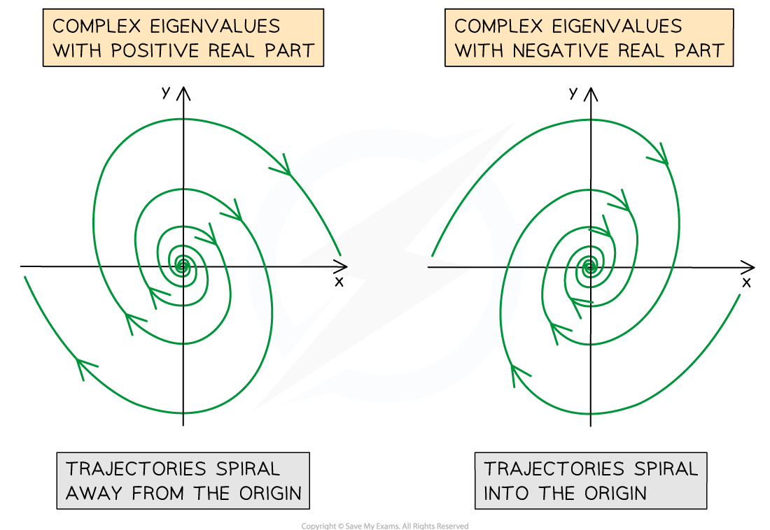
- You can determine the direction (clockwise or anticlockwise) of the trajectories by considering the values of and for points on the coordinate axes
- For example, consider the system
format('truetype')%3Bfont-weight%3Anormal%3Bfont-style%3Anormal%3B%7D%40font-face%7Bfont-family%3A'brack_sm2882ad605b1e27be87c7468'%3Bsrc%3Aurl(data%3Afont%2Ftruetype%3Bcharset%3Dutf-8%3Bbase64%2CAAEAAAAMAIAAAwBAT1MvMi7PH4UAAADMAAAATmNtYXA3kjw6AAABHAAAADxjdnQgAQYDiAAAAVgAAAASZ2x5ZkyYQ7YAAAFsAAAAkWhlYWQLyR8fAAACAAAAADZoaGVhAq0XCAAAAjgAAAAkaG10eDEjA%2FUAAAJcAAAADGxvY2EAAEKZAAACaAAAABBtYXhwBJsEcQAAAngAAAAgbmFtZW7QvZAAAAKYAAAB5XBvc3QArQBVAAAEgAAAACBwcmVwu5WEAAAABKAAAAAHAAACDAGQAAUAAAQABAAAAAAABAAEAAAAAAAAAQEAAAAAAAAAAAAAAAAAAAAAAAAAAAAAAAAAAAAAACAgICAAAAAg9AMD%2FP%2F8AAABVAABAAAAAAACAAEAAQAAABQAAwABAAAAFAAEACgAAAAGAAQAAQACI5wjn%2F%2F%2FAAAjnCOf%2F%2F%2FcZdxjAAEAAAAAAAAAAAFUAFQBAAArAIwAgACoAAcAAAACAAAAAADVAQEAAwAHAAAxMxEjFyM1M9XVq4CAAQHWqwABAAAAAABVAVgAAwAfGAGwAy%2BwADyxAgL1sAE8ALEDAD%2BwAjx8sQAG9bABPBEzESNVVQFY%2FqgAAQDXAAABLAFUAAMAIBgBsAUvsAE8sAI8sQAC9bADPACwAy%2BwAjyxAAH1sAE8EzMRI9dVVQFU%2FqwAAAAAAQAAAAEAAIsesexfDzz1AAMEAP%2F%2F%2F%2F%2FVre5k%2F%2F%2F%2F%2F9Wt7mT%2FgP%2F%2FAdYBWAAAAAoAAgABAAAAAAABAAABVP%2F%2FAAAXcP%2BA%2F4AB1gABAAAAAAAAAAAAAAAAAAAAAwDVAAABLAAAASwA1wAAAAAAAAAhAAAAWAAAAJEAAQAAAAMACgACAAAAAAACAIAEAAAAAAAEAABlAAAAAAAAABUBAgAAAAAAAAABACYAAAAAAAAAAAACAA4AJgAAAAAAAAADAEQANAAAAAAAAAAEACYAeAAAAAAAAAAFABYAngAAAAAAAAAGABMAtAAAAAAAAAAIABwAxwABAAAAAAABACYAAAABAAAAAAACAA4AJgABAAAAAAADAEQANAABAAAAAAAEACYAeAABAAAAAAAFABYAngABAAAAAAAGABMAtAABAAAAAAAIABwAxwADAAEECQABACYAAAADAAEECQACAA4AJgADAAEECQADAEQANAADAAEECQAEACYAeAADAAEECQAFABYAngADAAEECQAGABMAtAADAAEECQAIABwAxwBCAHIAYQBjAGsAZQB0AHMAIABzAG0AYQBsAGwAIABzAGkAegBlAFIAZQBnAHUAbABhAHIATQBhAHQAaABzACAARgBvAHIAIABNAG8AcgBlACAAQgByAGEAYwBrAGUAdABzACAAcwBtAGEAbABsACAAcwBpAHoAZQBCAHIAYQBjAGsAZQB0AHMAIABzAG0AYQBsAGwAIABzAGkAegBlAFYAZQByAHMAaQBvAG4AIAAyAC4AMEJyYWNrZXRzX3NtYWxsX3NpemUATQBhAHQAaABzACAARgBvAHIAIABNAG8AcgBlAAAAAAMAAAAAAAAAqgBVAAAAAAAAAAAAAAAAAAAAAAAAAAC5B%2F8AAo2FAA%3D%3D)format('truetype')%3Bfont-weight%3Anormal%3Bfont-style%3Anormal%3B%7D%40font-face%7Bfont-family%3A'bracketse552f5417ff4680c6b50499'%3Bsrc%3Aurl(data%3Afont%2Ftruetype%3Bcharset%3Dutf-8%3Bbase64%2CAAEAAAAMAIAAAwBAT1MvMi7RIisAAADMAAAATmNtYXBi7uzYAAABHAAAAExjdnQgBAkDLgAAAWgAAAASZ2x5Zo64f%2BkAAAF8AAABSWhlYWQLniGcAAACyAAAADZoaGVhBK4XLAAAAwAAAAAkaG10eCWq%2F90AAAMkAAAAFGxvY2EAABknAAADOAAAABhtYXhwBJIESAAAA1AAAAAgbmFtZRAA8I4AAANwAAAB3nBvc3QBwwDgAAAFUAAAACBwcmVwupWEAAAABXAAAAAHAAACggGQAAUAAAQABAAAAAAABAAEAAAAAAAAAQEAAAAAAAAAAAAAAAAAAAAAAAAAAAAAAAAAAAAAACAgICAAAAAg9AMEAAAAAAADgAAAAAAAAAACAAEAAQAAABQAAwABAAAAFAAEADgAAAAKAAgAAgACI5sjnSOeI6D%2F%2FwAAI5sjnSOeI6D%2F%2F9xm3GXcZdxkAAEAAAAAAAAAAAAAAAABVABWAQAALACoA4AAMgAHAAAAAgAAACoA1QNVAAMABwAANTMRIxMjETPV1auAgCoDK%2F0AAtUAAQAAAAABgAOAAAUAJBgBsAAvsAPFsQEC%2FbADELEEBP0AsQAAP7ABPLEEBj%2BwAzwwMTEzEAEjAFUBKyv%2BqwH8AYT%2BqgABAAAAAAGAA4AABQAmGAGwAC6wA8WxBQL9sAMQsQIE%2FQB8sQAGPxiwBTyxAwb2sAI8MDEREgEzABMBAVQr%2FtMCA4D91v6qAYQB%2FAAB%2F6wAAAEsA4AABQAnGAGwAC%2BwBzywA8WxAQL9sAMQsQQE%2FQCxAAA%2FsAE8sQQGP7ADPDAxISMSATMAASxVAf7UKwFVAfwBhP6rAAH%2FrAAAASwDgAAFACkYAbABL7AHPLAExbEAAv2wBBCxAwT9AHyxAQY%2FsAA8GLEEAD%2BwAzwwMRMzEAEjANdV%2FqsrASsDgP3V%2FqsBhgAAAAABAAAAAQAAeuTcpl8PPPUAAwQA%2F%2F%2F%2F%2F9Wt7o7%2F%2F%2F%2F%2F1a3ujv%2BsAAABgAOAAAAACgACAAEAAAAAAAEAAAOAAAAAABdw%2F6z%2FrAGAAAEAAAAAAAAAAAAAAAAAAAAFANUAAAEsAAABLAAAASz%2FrAEs%2F6wAAAAAAAAAJAAAAGgAAACzAAAA%2FQAAAUkAAQAAAAUACAACAAAAAAACAIAEAAAAAAAEAAA%2BAAAAAAAAABUBAgAAAAAAAAABACQAAAAAAAAAAAACAA4AJAAAAAAAAAADAEIAMgAAAAAAAAAEACQAdAAAAAAAAAAFABYAmAAAAAAAAAAGABIArgAAAAAAAAAIABwAwAABAAAAAAABACQAAAABAAAAAAACAA4AJAABAAAAAAADAEIAMgABAAAAAAAEACQAdAABAAAAAAAFABYAmAABAAAAAAAGABIArgABAAAAAAAIABwAwAADAAEECQABACQAAAADAAEECQACAA4AJAADAAEECQADAEIAMgADAAEECQAEACQAdAADAAEECQAFABYAmAADAAEECQAGABIArgADAAEECQAIABwAwABCAHIAYQBjAGsAZQB0AHMAIABmAHUAbABsACAAcwBpAHoAZQBSAGUAZwB1AGwAYQByAE0AYQB0AGgAcwAgAEYAbwByACAATQBvAHIAZQAgAEIAcgBhAGMAawBlAHQAcwAgAGYAdQBsAGwAIABzAGkAegBlAEIAcgBhAGMAawBlAHQAcwAgAGYAdQBsAGwAIABzAGkAegBlAFYAZQByAHMAaQBvAG4AIAAyAC4AMEJyYWNrZXRzX2Z1bGxfc2l6ZQBNAGEAdABoAHMAIABGAG8AcgAgAE0AbwByAGUAAAADAAAAAAAAAcAA4AAAAAAAAAAAAAAAAAAAAAAAAAAAuQf%2FAAGNhQA%3D)format('truetype')%3Bfont-weight%3Anormal%3Bfont-style%3Anormal%3B%7D%3C%2Fstyle%3E%3C%2Fdefs%3E%3Ctext%20font-family%3D%22math16d8888858ea6f9ebce8ea398ff%22%20font-size%3D%2212%22%20text-anchor%3D%22middle%22%20x%3D%225.5%22%20y%3D%2222%22%3E.%3C%2Ftext%3E%3Ctext%20font-family%3D%22Times%20New%20Roman%22%20font-size%3D%2218%22%20font-style%3D%22italic%22%20font-weight%3D%22bold%22%20text-anchor%3D%22middle%22%20x%3D%225.5%22%20y%3D%2233%22%3Ex%3C%2Ftext%3E%3Ctext%20font-family%3D%22math16d8888858ea6f9ebce8ea398ff%22%20font-size%3D%2216%22%20text-anchor%3D%22middle%22%20x%3D%2219.5%22%20y%3D%2233%22%3E%3D%3C%2Ftext%3E%3Ctext%20font-family%3D%22bracketse552f5417ff4680c6b50499%22%20font-size%3D%2218%22%20text-anchor%3D%22start%22%20x%3D%2229.5%22%20y%3D%2218%22%3E%26%23x239B%3B%3C%2Ftext%3E%3Ctext%20font-family%3D%22brack_sm2882ad605b1e27be87c7468%22%20font-size%3D%2218%22%20text-anchor%3D%22start%22%20x%3D%2229.5%22%20y%3D%2224%22%3E%26%23x239C%3B%3C%2Ftext%3E%3Ctext%20font-family%3D%22brack_sm2882ad605b1e27be87c7468%22%20font-size%3D%2218%22%20text-anchor%3D%22start%22%20x%3D%2229.5%22%20y%3D%2230%22%3E%26%23x239C%3B%3C%2Ftext%3E%3Ctext%20font-family%3D%22brack_sm2882ad605b1e27be87c7468%22%20font-size%3D%2218%22%20text-anchor%3D%22start%22%20x%3D%2229.5%22%20y%3D%2236%22%3E%26%23x239C%3B%3C%2Ftext%3E%3Ctext%20font-family%3D%22bracketse552f5417ff4680c6b50499%22%20font-size%3D%2218%22%20text-anchor%3D%22start%22%20x%3D%2229.5%22%20y%3D%2252%22%3E%26%23x239D%3B%3C%2Ftext%3E%3Ctext%20font-family%3D%22bracketse552f5417ff4680c6b50499%22%20font-size%3D%2218%22%20text-anchor%3D%22start%22%20x%3D%2283.5%22%20y%3D%2218%22%3E%26%23x239E%3B%3C%2Ftext%3E%3Ctext%20font-family%3D%22brack_sm2882ad605b1e27be87c7468%22%20font-size%3D%2218%22%20text-anchor%3D%22start%22%20x%3D%2283.5%22%20y%3D%2224%22%3E%26%23x239F%3B%3C%2Ftext%3E%3Ctext%20font-family%3D%22brack_sm2882ad605b1e27be87c7468%22%20font-size%3D%2218%22%20text-anchor%3D%22start%22%20x%3D%2283.5%22%20y%3D%2230%22%3E%26%23x239F%3B%3C%2Ftext%3E%3Ctext%20font-family%3D%22brack_sm2882ad605b1e27be87c7468%22%20font-size%3D%2218%22%20text-anchor%3D%22start%22%20x%3D%2283.5%22%20y%3D%2236%22%3E%26%23x239F%3B%3C%2Ftext%3E%3Ctext%20font-family%3D%22bracketse552f5417ff4680c6b50499%22%20font-size%3D%2218%22%20text-anchor%3D%22start%22%20x%3D%2283.5%22%20y%3D%2252%22%3E%26%23x23A0%3B%3C%2Ftext%3E%3Ctext%20font-family%3D%22Times%20New%20Roman%22%20font-size%3D%2218%22%20text-anchor%3D%22middle%22%20x%3D%2249.5%22%20y%3D%2219%22%3E1%3C%2Ftext%3E%3Ctext%20font-family%3D%22Times%20New%20Roman%22%20font-size%3D%2218%22%20text-anchor%3D%22middle%22%20x%3D%2273.5%22%20y%3D%2219%22%3E5%3C%2Ftext%3E%3Ctext%20font-family%3D%22math16d8888858ea6f9ebce8ea398ff%22%20font-size%3D%2216%22%20text-anchor%3D%22middle%22%20x%3D%2245.5%22%20y%3D%2245%22%3E%26%23x2212%3B%3C%2Ftext%3E%3Ctext%20font-family%3D%22Times%20New%20Roman%22%20font-size%3D%2218%22%20text-anchor%3D%22middle%22%20x%3D%2256.5%22%20y%3D%2245%22%3E2%3C%2Ftext%3E%3Ctext%20font-family%3D%22Times%20New%20Roman%22%20font-size%3D%2218%22%20text-anchor%3D%22middle%22%20x%3D%2273.5%22%20y%3D%2245%22%3E3%3C%2Ftext%3E%3Ctext%20font-family%3D%22Times%20New%20Roman%22%20font-size%3D%2218%22%20font-style%3D%22italic%22%20font-weight%3D%22bold%22%20text-anchor%3D%22middle%22%20x%3D%2294.5%22%20y%3D%2233%22%3Ex%3C%2Ftext%3E%3C%2Fsvg%3E)
- The eigenvalues of
format('truetype')%3Bfont-weight%3Anormal%3Bfont-style%3Anormal%3B%7D%40font-face%7Bfont-family%3A'brack_sm2882ad605b1e27be87c7468'%3Bsrc%3Aurl(data%3Afont%2Ftruetype%3Bcharset%3Dutf-8%3Bbase64%2CAAEAAAAMAIAAAwBAT1MvMi7PH4UAAADMAAAATmNtYXA3kjw6AAABHAAAADxjdnQgAQYDiAAAAVgAAAASZ2x5ZkyYQ7YAAAFsAAAAkWhlYWQLyR8fAAACAAAAADZoaGVhAq0XCAAAAjgAAAAkaG10eDEjA%2FUAAAJcAAAADGxvY2EAAEKZAAACaAAAABBtYXhwBJsEcQAAAngAAAAgbmFtZW7QvZAAAAKYAAAB5XBvc3QArQBVAAAEgAAAACBwcmVwu5WEAAAABKAAAAAHAAACDAGQAAUAAAQABAAAAAAABAAEAAAAAAAAAQEAAAAAAAAAAAAAAAAAAAAAAAAAAAAAAAAAAAAAACAgICAAAAAg9AMD%2FP%2F8AAABVAABAAAAAAACAAEAAQAAABQAAwABAAAAFAAEACgAAAAGAAQAAQACI5wjn%2F%2F%2FAAAjnCOf%2F%2F%2FcZdxjAAEAAAAAAAAAAAFUAFQBAAArAIwAgACoAAcAAAACAAAAAADVAQEAAwAHAAAxMxEjFyM1M9XVq4CAAQHWqwABAAAAAABVAVgAAwAfGAGwAy%2BwADyxAgL1sAE8ALEDAD%2BwAjx8sQAG9bABPBEzESNVVQFY%2FqgAAQDXAAABLAFUAAMAIBgBsAUvsAE8sAI8sQAC9bADPACwAy%2BwAjyxAAH1sAE8EzMRI9dVVQFU%2FqwAAAAAAQAAAAEAAIsesexfDzz1AAMEAP%2F%2F%2F%2F%2FVre5k%2F%2F%2F%2F%2F9Wt7mT%2FgP%2F%2FAdYBWAAAAAoAAgABAAAAAAABAAABVP%2F%2FAAAXcP%2BA%2F4AB1gABAAAAAAAAAAAAAAAAAAAAAwDVAAABLAAAASwA1wAAAAAAAAAhAAAAWAAAAJEAAQAAAAMACgACAAAAAAACAIAEAAAAAAAEAABlAAAAAAAAABUBAgAAAAAAAAABACYAAAAAAAAAAAACAA4AJgAAAAAAAAADAEQANAAAAAAAAAAEACYAeAAAAAAAAAAFABYAngAAAAAAAAAGABMAtAAAAAAAAAAIABwAxwABAAAAAAABACYAAAABAAAAAAACAA4AJgABAAAAAAADAEQANAABAAAAAAAEACYAeAABAAAAAAAFABYAngABAAAAAAAGABMAtAABAAAAAAAIABwAxwADAAEECQABACYAAAADAAEECQACAA4AJgADAAEECQADAEQANAADAAEECQAEACYAeAADAAEECQAFABYAngADAAEECQAGABMAtAADAAEECQAIABwAxwBCAHIAYQBjAGsAZQB0AHMAIABzAG0AYQBsAGwAIABzAGkAegBlAFIAZQBnAHUAbABhAHIATQBhAHQAaABzACAARgBvAHIAIABNAG8AcgBlACAAQgByAGEAYwBrAGUAdABzACAAcwBtAGEAbABsACAAcwBpAHoAZQBCAHIAYQBjAGsAZQB0AHMAIABzAG0AYQBsAGwAIABzAGkAegBlAFYAZQByAHMAaQBvAG4AIAAyAC4AMEJyYWNrZXRzX3NtYWxsX3NpemUATQBhAHQAaABzACAARgBvAHIAIABNAG8AcgBlAAAAAAMAAAAAAAAAqgBVAAAAAAAAAAAAAAAAAAAAAAAAAAC5B%2F8AAo2FAA%3D%3D)format('truetype')%3Bfont-weight%3Anormal%3Bfont-style%3Anormal%3B%7D%40font-face%7Bfont-family%3A'bracketse552f5417ff4680c6b50499'%3Bsrc%3Aurl(data%3Afont%2Ftruetype%3Bcharset%3Dutf-8%3Bbase64%2CAAEAAAAMAIAAAwBAT1MvMi7RIisAAADMAAAATmNtYXBi7uzYAAABHAAAAExjdnQgBAkDLgAAAWgAAAASZ2x5Zo64f%2BkAAAF8AAABSWhlYWQLniGcAAACyAAAADZoaGVhBK4XLAAAAwAAAAAkaG10eCWq%2F90AAAMkAAAAFGxvY2EAABknAAADOAAAABhtYXhwBJIESAAAA1AAAAAgbmFtZRAA8I4AAANwAAAB3nBvc3QBwwDgAAAFUAAAACBwcmVwupWEAAAABXAAAAAHAAACggGQAAUAAAQABAAAAAAABAAEAAAAAAAAAQEAAAAAAAAAAAAAAAAAAAAAAAAAAAAAAAAAAAAAACAgICAAAAAg9AMEAAAAAAADgAAAAAAAAAACAAEAAQAAABQAAwABAAAAFAAEADgAAAAKAAgAAgACI5sjnSOeI6D%2F%2FwAAI5sjnSOeI6D%2F%2F9xm3GXcZdxkAAEAAAAAAAAAAAAAAAABVABWAQAALACoA4AAMgAHAAAAAgAAACoA1QNVAAMABwAANTMRIxMjETPV1auAgCoDK%2F0AAtUAAQAAAAABgAOAAAUAJBgBsAAvsAPFsQEC%2FbADELEEBP0AsQAAP7ABPLEEBj%2BwAzwwMTEzEAEjAFUBKyv%2BqwH8AYT%2BqgABAAAAAAGAA4AABQAmGAGwAC6wA8WxBQL9sAMQsQIE%2FQB8sQAGPxiwBTyxAwb2sAI8MDEREgEzABMBAVQr%2FtMCA4D91v6qAYQB%2FAAB%2F6wAAAEsA4AABQAnGAGwAC%2BwBzywA8WxAQL9sAMQsQQE%2FQCxAAA%2FsAE8sQQGP7ADPDAxISMSATMAASxVAf7UKwFVAfwBhP6rAAH%2FrAAAASwDgAAFACkYAbABL7AHPLAExbEAAv2wBBCxAwT9AHyxAQY%2FsAA8GLEEAD%2BwAzwwMRMzEAEjANdV%2FqsrASsDgP3V%2FqsBhgAAAAABAAAAAQAAeuTcpl8PPPUAAwQA%2F%2F%2F%2F%2F9Wt7o7%2F%2F%2F%2F%2F1a3ujv%2BsAAABgAOAAAAACgACAAEAAAAAAAEAAAOAAAAAABdw%2F6z%2FrAGAAAEAAAAAAAAAAAAAAAAAAAAFANUAAAEsAAABLAAAASz%2FrAEs%2F6wAAAAAAAAAJAAAAGgAAACzAAAA%2FQAAAUkAAQAAAAUACAACAAAAAAACAIAEAAAAAAAEAAA%2BAAAAAAAAABUBAgAAAAAAAAABACQAAAAAAAAAAAACAA4AJAAAAAAAAAADAEIAMgAAAAAAAAAEACQAdAAAAAAAAAAFABYAmAAAAAAAAAAGABIArgAAAAAAAAAIABwAwAABAAAAAAABACQAAAABAAAAAAACAA4AJAABAAAAAAADAEIAMgABAAAAAAAEACQAdAABAAAAAAAFABYAmAABAAAAAAAGABIArgABAAAAAAAIABwAwAADAAEECQABACQAAAADAAEECQACAA4AJAADAAEECQADAEIAMgADAAEECQAEACQAdAADAAEECQAFABYAmAADAAEECQAGABIArgADAAEECQAIABwAwABCAHIAYQBjAGsAZQB0AHMAIABmAHUAbABsACAAcwBpAHoAZQBSAGUAZwB1AGwAYQByAE0AYQB0AGgAcwAgAEYAbwByACAATQBvAHIAZQAgAEIAcgBhAGMAawBlAHQAcwAgAGYAdQBsAGwAIABzAGkAegBlAEIAcgBhAGMAawBlAHQAcwAgAGYAdQBsAGwAIABzAGkAegBlAFYAZQByAHMAaQBvAG4AIAAyAC4AMEJyYWNrZXRzX2Z1bGxfc2l6ZQBNAGEAdABoAHMAIABGAG8AcgAgAE0AbwByAGUAAAADAAAAAAAAAcAA4AAAAAAAAAAAAAAAAAAAAAAAAAAAuQf%2FAAGNhQA%3D)format('truetype')%3Bfont-weight%3Anormal%3Bfont-style%3Anormal%3B%7D%3C%2Fstyle%3E%3C%2Fdefs%3E%3Ctext%20font-family%3D%22bracketse552f5417ff4680c6b50499%22%20font-size%3D%2218%22%20text-anchor%3D%22start%22%20x%3D%221.5%22%20y%3D%2218%22%3E%26%23x239B%3B%3C%2Ftext%3E%3Ctext%20font-family%3D%22brack_sm2882ad605b1e27be87c7468%22%20font-size%3D%2218%22%20text-anchor%3D%22start%22%20x%3D%221.5%22%20y%3D%2224%22%3E%26%23x239C%3B%3C%2Ftext%3E%3Ctext%20font-family%3D%22brack_sm2882ad605b1e27be87c7468%22%20font-size%3D%2218%22%20text-anchor%3D%22start%22%20x%3D%221.5%22%20y%3D%2230%22%3E%26%23x239C%3B%3C%2Ftext%3E%3Ctext%20font-family%3D%22brack_sm2882ad605b1e27be87c7468%22%20font-size%3D%2218%22%20text-anchor%3D%22start%22%20x%3D%221.5%22%20y%3D%2236%22%3E%26%23x239C%3B%3C%2Ftext%3E%3Ctext%20font-family%3D%22bracketse552f5417ff4680c6b50499%22%20font-size%3D%2218%22%20text-anchor%3D%22start%22%20x%3D%221.5%22%20y%3D%2252%22%3E%26%23x239D%3B%3C%2Ftext%3E%3Ctext%20font-family%3D%22bracketse552f5417ff4680c6b50499%22%20font-size%3D%2218%22%20text-anchor%3D%22start%22%20x%3D%2255.5%22%20y%3D%2218%22%3E%26%23x239E%3B%3C%2Ftext%3E%3Ctext%20font-family%3D%22brack_sm2882ad605b1e27be87c7468%22%20font-size%3D%2218%22%20text-anchor%3D%22start%22%20x%3D%2255.5%22%20y%3D%2224%22%3E%26%23x239F%3B%3C%2Ftext%3E%3Ctext%20font-family%3D%22brack_sm2882ad605b1e27be87c7468%22%20font-size%3D%2218%22%20text-anchor%3D%22start%22%20x%3D%2255.5%22%20y%3D%2230%22%3E%26%23x239F%3B%3C%2Ftext%3E%3Ctext%20font-family%3D%22brack_sm2882ad605b1e27be87c7468%22%20font-size%3D%2218%22%20text-anchor%3D%22start%22%20x%3D%2255.5%22%20y%3D%2236%22%3E%26%23x239F%3B%3C%2Ftext%3E%3Ctext%20font-family%3D%22bracketse552f5417ff4680c6b50499%22%20font-size%3D%2218%22%20text-anchor%3D%22start%22%20x%3D%2255.5%22%20y%3D%2252%22%3E%26%23x23A0%3B%3C%2Ftext%3E%3Ctext%20font-family%3D%22Times%20New%20Roman%22%20font-size%3D%2218%22%20text-anchor%3D%22middle%22%20x%3D%2215.5%22%20y%3D%2219%22%3E1%3C%2Ftext%3E%3Ctext%20font-family%3D%22math1da40657c9fece7e48d30af42d3%22%20font-size%3D%2216%22%20text-anchor%3D%22middle%22%20x%3D%2234.5%22%20y%3D%2219%22%3E%26%23x2212%3B%3C%2Ftext%3E%3Ctext%20font-family%3D%22Times%20New%20Roman%22%20font-size%3D%2218%22%20text-anchor%3D%22middle%22%20x%3D%2245.5%22%20y%3D%2219%22%3E5%3C%2Ftext%3E%3Ctext%20font-family%3D%22Times%20New%20Roman%22%20font-size%3D%2218%22%20text-anchor%3D%22middle%22%20x%3D%2215.5%22%20y%3D%2245%22%3E2%3C%2Ftext%3E%3Ctext%20font-family%3D%22Times%20New%20Roman%22%20font-size%3D%2218%22%20text-anchor%3D%22middle%22%20x%3D%2238.5%22%20y%3D%2245%22%3E3%3C%2Ftext%3E%3C%2Fsvg%3E) are
are format('truetype')%3Bfont-weight%3Anormal%3Bfont-style%3Anormal%3B%7D%3C%2Fstyle%3E%3C%2Fdefs%3E%3Ctext%20font-family%3D%22Times%20New%20Roman%22%20font-size%3D%2218%22%20text-anchor%3D%22middle%22%20x%3D%224.5%22%20y%3D%2216%22%3E2%3C%2Ftext%3E%3Ctext%20font-family%3D%22math117e62166fc8586dfa4d1bc0e17%22%20font-size%3D%2216%22%20text-anchor%3D%22middle%22%20x%3D%2217.5%22%20y%3D%2216%22%3E%2B%3C%2Ftext%3E%3Ctext%20font-family%3D%22Times%20New%20Roman%22%20font-size%3D%2218%22%20text-anchor%3D%22middle%22%20x%3D%2230.5%22%20y%3D%2216%22%3E3%3C%2Ftext%3E%3Ctext%20font-family%3D%22Times%20New%20Roman%22%20font-size%3D%2218%22%20text-anchor%3D%22middle%22%20x%3D%2237.5%22%20y%3D%2216%22%3Ei%3C%2Ftext%3E%3C%2Fsvg%3E) and
and format('truetype')%3Bfont-weight%3Anormal%3Bfont-style%3Anormal%3B%7D%3C%2Fstyle%3E%3C%2Fdefs%3E%3Ctext%20font-family%3D%22Times%20New%20Roman%22%20font-size%3D%2218%22%20text-anchor%3D%22middle%22%20x%3D%224.5%22%20y%3D%2216%22%3E2%3C%2Ftext%3E%3Ctext%20font-family%3D%22math1da40657c9fece7e48d30af42d3%22%20font-size%3D%2216%22%20text-anchor%3D%22middle%22%20x%3D%2217.5%22%20y%3D%2216%22%3E%26%23x2212%3B%3C%2Ftext%3E%3Ctext%20font-family%3D%22Times%20New%20Roman%22%20font-size%3D%2218%22%20text-anchor%3D%22middle%22%20x%3D%2230.5%22%20y%3D%2216%22%3E3%3C%2Ftext%3E%3Ctext%20font-family%3D%22Times%20New%20Roman%22%20font-size%3D%2218%22%20text-anchor%3D%22middle%22%20x%3D%2237.5%22%20y%3D%2216%22%3Ei%3C%2Ftext%3E%3C%2Fsvg%3E) , so the trajectories will be spirals
, so the trajectories will be spirals
- The eigenvalues of
- For example, consider the system
- Because the real part of the eigenvalues
%3C%2Fmo%3E%3C%2Fmath%3E--%3E%3Cdefs%3E%3Cstyle%20type%3D%22text%2Fcss%22%3E%40font-face%7Bfont-family%3A'round_brackets18549f92a457f2409'%3Bsrc%3Aurl(data%3Afont%2Ftruetype%3Bcharset%3Dutf-8%3Bbase64%2CAAEAAAAMAIAAAwBAT1MvMjwHLFQAAADMAAAATmNtYXDf7xCrAAABHAAAADxjdnQgBAkDLgAAAVgAAAASZ2x5ZmAOz2cAAAFsAAABJGhlYWQOKih8AAACkAAAADZoaGVhCvgVwgAAAsgAAAAkaG10eCA6AAIAAALsAAAADGxvY2EAAARLAAAC%2BAAAABBtYXhwBIgEWQAAAwgAAAAgbmFtZXHR30MAAAMoAAACOXBvc3QDogHPAAAFZAAAACBwcmVwupWEAAAABYQAAAAHAAAGcgGQAAUAAAgACAAAAAAACAAIAAAAAAAAAQIAAAAAAAAAAAAAAAAAAAAAAAAAAAAAAAAAAAAAACAgICAAAAAo8AMGe%2F57AAAHPgGyAAAAAAACAAEAAQAAABQAAwABAAAAFAAEACgAAAAGAAQAAQACACgAKf%2F%2FAAAAKAAp%2F%2F%2F%2F2f%2FZAAEAAAAAAAAAAAFUAFYBAAAsAKgDgAAyAAcAAAACAAAAKgDVA1UAAwAHAAA1MxEjEyMRM9XVq4CAKgMr%2FQAC1QABAAD%2B0AIgBtAACQBNGAGwChCwA9SwAxCwAtSwChCwBdSwBRCwANSwAxCwBzywAhCwCDwAsAoQsAPUsAMQsAfUsAoQsAXUsAoQsADUsAMQsAI8sAcQsAg8MTAREAEzABEQASMAAZCQ%2FnABkJD%2BcALQ%2FZD%2BcAGQAnACcAGQ%2FnAAAQAA%2FtACIAbQAAkATRgBsAoQsAPUsAMQsALUsAoQsAXUsAUQsADUsAMQsAc8sAIQsAg8ALAKELAD1LADELAH1LAKELAF1LAKELAA1LADELACPLAHELAIPDEwARABIwAREAEzAAIg%2FnCQAZD%2BcJABkALQ%2FZD%2BcAGQAnACcAGQ%2FnAAAQAAAAEAAPW2NYFfDzz1AAMIAP%2F%2F%2F%2F%2FVre7u%2F%2F%2F%2F%2F9Wt7u4AAP7QA7cG0AAAAAoAAgABAAAAAAABAAAHPv5OAAAXcAAA%2F%2F4DtwABAAAAAAAAAAAAAAAAAAAAAwDVAAACIAAAAiAAAAAAAAAAAAAkAAAAowAAASQAAQAAAAMACgACAAAAAAACAIAEAAAAAAAEAABNAAAAAAAAABUBAgAAAAAAAAABAD4AAAAAAAAAAAACAA4APgAAAAAAAAADAFwATAAAAAAAAAAEAD4AqAAAAAAAAAAFABYA5gAAAAAAAAAGAB8A%2FAAAAAAAAAAIABwBGwABAAAAAAABAD4AAAABAAAAAAACAA4APgABAAAAAAADAFwATAABAAAAAAAEAD4AqAABAAAAAAAFABYA5gABAAAAAAAGAB8A%2FAABAAAAAAAIABwBGwADAAEECQABAD4AAAADAAEECQACAA4APgADAAEECQADAFwATAADAAEECQAEAD4AqAADAAEECQAFABYA5gADAAEECQAGAB8A%2FAADAAEECQAIABwBGwBSAG8AdQBuAGQAIABiAHIAYQBjAGsAZQB0AHMAIAB3AGkAdABoACAAYQBzAGMAZQBuAHQAIAAxADgANQA0AFIAZQBnAHUAbABhAHIATQBhAHQAaABzACAARgBvAHIAIABNAG8AcgBlACAAUgBvAHUAbgBkACAAYgByAGEAYwBrAGUAdABzACAAdwBpAHQAaAAgAGEAcwBjAGUAbgB0ACAAMQA4ADUANABSAG8AdQBuAGQAIABiAHIAYQBjAGsAZQB0AHMAIAB3AGkAdABoACAAYQBzAGMAZQBuAHQAIAAxADgANQA0AFYAZQByAHMAaQBvAG4AIAAyAC4AMFJvdW5kX2JyYWNrZXRzX3dpdGhfYXNjZW50XzE4NTQATQBhAHQAaABzACAARgBvAHIAIABNAG8AcgBlAAAAAAMAAAAAAAADnwHPAAAAAAAAAAAAAAAAAAAAAAAAAAC5B%2F8AAY2FAA%3D%3D)format('truetype')%3Bfont-weight%3Anormal%3Bfont-style%3Anormal%3B%7D%3C%2Fstyle%3E%3C%2Fdefs%3E%3Ctext%20font-family%3D%22round_brackets18549f92a457f2409%22%20font-size%3D%2218%22%20text-anchor%3D%22middle%22%20x%3D%223.5%22%20y%3D%2216%22%3E(%3C%2Ftext%3E%3Ctext%20font-family%3D%22Times%20New%20Roman%22%20font-size%3D%2218%22%20text-anchor%3D%22middle%22%20x%3D%2210.5%22%20y%3D%2216%22%3E2%3C%2Ftext%3E%3Ctext%20font-family%3D%22round_brackets18549f92a457f2409%22%20font-size%3D%2218%22%20text-anchor%3D%22middle%22%20x%3D%2217.5%22%20y%3D%2216%22%3E)%3C%2Ftext%3E%3C%2Fsvg%3E) is positive, the trajectories will spiral away from the origin
is positive, the trajectories will spiral away from the origin - When and ,
%3C%2Fmo%3E%3Cmo%3E%2B%3C%2Fmo%3E%3Cmn%3E5%3C%2Fmn%3E%3Cmo%3E(%3C%2Fmo%3E%3Cmn%3E0%3C%2Fmn%3E%3Cmo%3E)%3C%2Fmo%3E%3Cmo%3E%3D%3C%2Fmo%3E%3Cmn%3E1%3C%2Fmn%3E%3C%2Fmath%3E--%3E%3Cdefs%3E%3Cstyle%20type%3D%22text%2Fcss%22%3E%40font-face%7Bfont-family%3A'math1564b4c0e54101ac57a0cb68c16'%3Bsrc%3Aurl(data%3Afont%2Ftruetype%3Bcharset%3Dutf-8%3Bbase64%2CAAEAAAAMAIAAAwBAT1MvMi7iBBMAAADMAAAATmNtYXDEvmKUAAABHAAAADxjdnQgDVUNBwAAAVgAAAA6Z2x5ZoPi2VsAAAGUAAABK2hlYWQQC2qxAAACwAAAADZoaGVhCGsXSAAAAvgAAAAkaG10eE2rRkcAAAMcAAAADGxvY2EAHTwYAAADKAAAABBtYXhwBT0FPgAAAzgAAAAgbmFtZaBxlY4AAANYAAABn3Bvc3QB9wD6AAAE%2BAAAACBwcmVwa1uragAABRgAAAAUAAADSwGQAAUAAAQABAAAAAAABAAEAAAAAAAAAQEAAAAAAAAAAAAAAAAAAAAAAAAAAAAAAAAAAAAAACAgICAAAAAg1UADev96AAAD6ACWAAAAAAACAAEAAQAAABQAAwABAAAAFAAEACgAAAAGAAQAAQACACsAPf%2F%2FAAAAKwA9%2F%2F%2F%2F1v%2FFAAEAAAAAAAAAAAFUAywAgAEAAFYAKgJYAh4BDgEsAiwAWgGAAoAAoADUAIAAAAAAAAAAKwBVAIAAqwDVAQABKwAHAAAAAgBVAAADAAOrAAMABwAAMxEhESUhESFVAqv9qwIA%2FgADq%2FxVVQMAAAEAgABVAtUCqwALAEkBGLIMAQEUExCxAAP2sQEE9bAKPLEDBfWwCDyxBQT1sAY8sQ0D5gCxAAATELEBBuSxAQETELAFPLEDBOWxCwX1sAc8sQkE5TEwEyERMxEhFSERIxEhgAEAVQEA%2FwBV%2FwABqwEA%2FwBW%2FwABAAACAIAA6wLVAhUAAwAHAGUYAbAIELAG1LAGELAF1LAIELAB1LABELAA1LAGELAHPLAFELAEPLABELACPLAAELADPACwCBCwBtSwBhCwB9SwBxCwAdSwARCwAtSwBhCwBTywBxCwBDywARCwADywAhCwAzwxMBMhNSEdASE1gAJV%2FasCVQHAVdVVVQAAAQAAAAEAANV4zkFfDzz1AAMEAP%2F%2F%2F%2F%2FWOhNz%2F%2F%2F%2F%2F9Y6E3MAAP8gBIADqwAAAAoAAgABAAAAAAABAAAD6P9qAAAXcAAA%2F7YEgAABAAAAAAAAAAAAAAAAAAAAAwNSAFUDVgCAA1YAgAAAAAAAAAAoAAAAoQAAASsAAQAAAAMAXgAFAAAAAAACAIAEAAAAAAAEAADeAAAAAAAAABUBAgAAAAAAAAABABIAAAAAAAAAAAACAA4AEgAAAAAAAAADADAAIAAAAAAAAAAEABIAUAAAAAAAAAAFABYAYgAAAAAAAAAGAAkAeAAAAAAAAAAIABwAgQABAAAAAAABABIAAAABAAAAAAACAA4AEgABAAAAAAADADAAIAABAAAAAAAEABIAUAABAAAAAAAFABYAYgABAAAAAAAGAAkAeAABAAAAAAAIABwAgQADAAEECQABABIAAAADAAEECQACAA4AEgADAAEECQADADAAIAADAAEECQAEABIAUAADAAEECQAFABYAYgADAAEECQAGAAkAeAADAAEECQAIABwAgQBNAGEAdABoACAARgBvAG4AdABSAGUAZwB1AGwAYQByAE0AYQB0AGgAcwAgAEYAbwByACAATQBvAHIAZQAgAE0AYQB0AGgAIABGAG8AbgB0AE0AYQB0AGgAIABGAG8AbgB0AFYAZQByAHMAaQBvAG4AIAAxAC4AME1hdGhfRm9udABNAGEAdABoAHMAIABGAG8AcgAgAE0AbwByAGUAAAMAAAAAAAAB9AD6AAAAAAAAAAAAAAAAAAAAAAAAAAC5BxEAAI2FGACyAAAAFRQTsQABPw%3D%3D)format('truetype')%3Bfont-weight%3Anormal%3Bfont-style%3Anormal%3B%7D%40font-face%7Bfont-family%3A'round_brackets18549f92a457f2409'%3Bsrc%3Aurl(data%3Afont%2Ftruetype%3Bcharset%3Dutf-8%3Bbase64%2CAAEAAAAMAIAAAwBAT1MvMjwHLFQAAADMAAAATmNtYXDf7xCrAAABHAAAADxjdnQgBAkDLgAAAVgAAAASZ2x5ZmAOz2cAAAFsAAABJGhlYWQOKih8AAACkAAAADZoaGVhCvgVwgAAAsgAAAAkaG10eCA6AAIAAALsAAAADGxvY2EAAARLAAAC%2BAAAABBtYXhwBIgEWQAAAwgAAAAgbmFtZXHR30MAAAMoAAACOXBvc3QDogHPAAAFZAAAACBwcmVwupWEAAAABYQAAAAHAAAGcgGQAAUAAAgACAAAAAAACAAIAAAAAAAAAQIAAAAAAAAAAAAAAAAAAAAAAAAAAAAAAAAAAAAAACAgICAAAAAo8AMGe%2F57AAAHPgGyAAAAAAACAAEAAQAAABQAAwABAAAAFAAEACgAAAAGAAQAAQACACgAKf%2F%2FAAAAKAAp%2F%2F%2F%2F2f%2FZAAEAAAAAAAAAAAFUAFYBAAAsAKgDgAAyAAcAAAACAAAAKgDVA1UAAwAHAAA1MxEjEyMRM9XVq4CAKgMr%2FQAC1QABAAD%2B0AIgBtAACQBNGAGwChCwA9SwAxCwAtSwChCwBdSwBRCwANSwAxCwBzywAhCwCDwAsAoQsAPUsAMQsAfUsAoQsAXUsAoQsADUsAMQsAI8sAcQsAg8MTAREAEzABEQASMAAZCQ%2FnABkJD%2BcALQ%2FZD%2BcAGQAnACcAGQ%2FnAAAQAA%2FtACIAbQAAkATRgBsAoQsAPUsAMQsALUsAoQsAXUsAUQsADUsAMQsAc8sAIQsAg8ALAKELAD1LADELAH1LAKELAF1LAKELAA1LADELACPLAHELAIPDEwARABIwAREAEzAAIg%2FnCQAZD%2BcJABkALQ%2FZD%2BcAGQAnACcAGQ%2FnAAAQAAAAEAAPW2NYFfDzz1AAMIAP%2F%2F%2F%2F%2FVre7u%2F%2F%2F%2F%2F9Wt7u4AAP7QA7cG0AAAAAoAAgABAAAAAAABAAAHPv5OAAAXcAAA%2F%2F4DtwABAAAAAAAAAAAAAAAAAAAAAwDVAAACIAAAAiAAAAAAAAAAAAAkAAAAowAAASQAAQAAAAMACgACAAAAAAACAIAEAAAAAAAEAABNAAAAAAAAABUBAgAAAAAAAAABAD4AAAAAAAAAAAACAA4APgAAAAAAAAADAFwATAAAAAAAAAAEAD4AqAAAAAAAAAAFABYA5gAAAAAAAAAGAB8A%2FAAAAAAAAAAIABwBGwABAAAAAAABAD4AAAABAAAAAAACAA4APgABAAAAAAADAFwATAABAAAAAAAEAD4AqAABAAAAAAAFABYA5gABAAAAAAAGAB8A%2FAABAAAAAAAIABwBGwADAAEECQABAD4AAAADAAEECQACAA4APgADAAEECQADAFwATAADAAEECQAEAD4AqAADAAEECQAFABYA5gADAAEECQAGAB8A%2FAADAAEECQAIABwBGwBSAG8AdQBuAGQAIABiAHIAYQBjAGsAZQB0AHMAIAB3AGkAdABoACAAYQBzAGMAZQBuAHQAIAAxADgANQA0AFIAZQBnAHUAbABhAHIATQBhAHQAaABzACAARgBvAHIAIABNAG8AcgBlACAAUgBvAHUAbgBkACAAYgByAGEAYwBrAGUAdABzACAAdwBpAHQAaAAgAGEAcwBjAGUAbgB0ACAAMQA4ADUANABSAG8AdQBuAGQAIABiAHIAYQBjAGsAZQB0AHMAIAB3AGkAdABoACAAYQBzAGMAZQBuAHQAIAAxADgANQA0AFYAZQByAHMAaQBvAG4AIAAyAC4AMFJvdW5kX2JyYWNrZXRzX3dpdGhfYXNjZW50XzE4NTQATQBhAHQAaABzACAARgBvAHIAIABNAG8AcgBlAAAAAAMAAAAAAAADnwHPAAAAAAAAAAAAAAAAAAAAAAAAAAC5B%2F8AAY2FAA%3D%3D)format('truetype')%3Bfont-weight%3Anormal%3Bfont-style%3Anormal%3B%7D%3C%2Fstyle%3E%3C%2Fdefs%3E%3Cline%20stroke%3D%22%23000000%22%20stroke-linecap%3D%22square%22%20stroke-width%3D%221%22%20x1%3D%222.5%22%20x2%3D%2225.5%22%20y1%3D%2223.5%22%20y2%3D%2223.5%22%2F%3E%3Ctext%20font-family%3D%22Times%20New%20Roman%22%20font-size%3D%2218%22%20text-anchor%3D%22middle%22%20x%3D%229.5%22%20y%3D%2216%22%3Ed%3C%2Ftext%3E%3Ctext%20font-family%3D%22Times%20New%20Roman%22%20font-size%3D%2218%22%20font-style%3D%22italic%22%20text-anchor%3D%22middle%22%20x%3D%2218.5%22%20y%3D%2216%22%3Ex%3C%2Ftext%3E%3Ctext%20font-family%3D%22Times%20New%20Roman%22%20font-size%3D%2218%22%20text-anchor%3D%22middle%22%20x%3D%2211.5%22%20y%3D%2241%22%3Ed%3C%2Ftext%3E%3Ctext%20font-family%3D%22Times%20New%20Roman%22%20font-size%3D%2218%22%20font-style%3D%22italic%22%20text-anchor%3D%22middle%22%20x%3D%2218.5%22%20y%3D%2241%22%3Et%3C%2Ftext%3E%3Ctext%20font-family%3D%22math1564b4c0e54101ac57a0cb68c16%22%20font-size%3D%2216%22%20text-anchor%3D%22middle%22%20x%3D%2236.5%22%20y%3D%2230%22%3E%3D%3C%2Ftext%3E%3Ctext%20font-family%3D%22Times%20New%20Roman%22%20font-size%3D%2218%22%20text-anchor%3D%22middle%22%20x%3D%2249.5%22%20y%3D%2230%22%3E1%3C%2Ftext%3E%3Ctext%20font-family%3D%22round_brackets18549f92a457f2409%22%20font-size%3D%2218%22%20text-anchor%3D%22middle%22%20x%3D%2257.5%22%20y%3D%2230%22%3E(%3C%2Ftext%3E%3Ctext%20font-family%3D%22Times%20New%20Roman%22%20font-size%3D%2218%22%20text-anchor%3D%22middle%22%20x%3D%2264.5%22%20y%3D%2230%22%3E1%3C%2Ftext%3E%3Ctext%20font-family%3D%22round_brackets18549f92a457f2409%22%20font-size%3D%2218%22%20text-anchor%3D%22middle%22%20x%3D%2271.5%22%20y%3D%2230%22%3E)%3C%2Ftext%3E%3Ctext%20font-family%3D%22math1564b4c0e54101ac57a0cb68c16%22%20font-size%3D%2216%22%20text-anchor%3D%22middle%22%20x%3D%2283.5%22%20y%3D%2230%22%3E%2B%3C%2Ftext%3E%3Ctext%20font-family%3D%22Times%20New%20Roman%22%20font-size%3D%2218%22%20text-anchor%3D%22middle%22%20x%3D%2296.5%22%20y%3D%2230%22%3E5%3C%2Ftext%3E%3Ctext%20font-family%3D%22round_brackets18549f92a457f2409%22%20font-size%3D%2218%22%20text-anchor%3D%22middle%22%20x%3D%22104.5%22%20y%3D%2230%22%3E(%3C%2Ftext%3E%3Ctext%20font-family%3D%22Times%20New%20Roman%22%20font-size%3D%2218%22%20text-anchor%3D%22middle%22%20x%3D%22111.5%22%20y%3D%2230%22%3E0%3C%2Ftext%3E%3Ctext%20font-family%3D%22round_brackets18549f92a457f2409%22%20font-size%3D%2218%22%20text-anchor%3D%22middle%22%20x%3D%22118.5%22%20y%3D%2230%22%3E)%3C%2Ftext%3E%3Ctext%20font-family%3D%22math1564b4c0e54101ac57a0cb68c16%22%20font-size%3D%2216%22%20text-anchor%3D%22middle%22%20x%3D%22130.5%22%20y%3D%2230%22%3E%3D%3C%2Ftext%3E%3Ctext%20font-family%3D%22Times%20New%20Roman%22%20font-size%3D%2218%22%20text-anchor%3D%22middle%22%20x%3D%22143.5%22%20y%3D%2230%22%3E1%3C%2Ftext%3E%3C%2Fsvg%3E) and
and %3C%2Fmo%3E%3Cmo%3E%2B%3C%2Fmo%3E%3Cmn%3E3%3C%2Fmn%3E%3Cmo%3E(%3C%2Fmo%3E%3Cmn%3E0%3C%2Fmn%3E%3Cmo%3E)%3C%2Fmo%3E%3Cmo%3E%3D%3C%2Fmo%3E%3Cmo%3E-%3C%2Fmo%3E%3Cmn%3E2%3C%2Fmn%3E%3C%2Fmath%3E--%3E%3Cdefs%3E%3Cstyle%20type%3D%22text%2Fcss%22%3E%40font-face%7Bfont-family%3A'math190bc3972c7934354efb2af01e7'%3Bsrc%3Aurl(data%3Afont%2Ftruetype%3Bcharset%3Dutf-8%3Bbase64%2CAAEAAAAMAIAAAwBAT1MvMi7iBBMAAADMAAAATmNtYXDEvmKUAAABHAAAAERjdnQgDVUNBwAAAWAAAAA6Z2x5ZoPi2VsAAAGcAAABdWhlYWQQC2qxAAADFAAAADZoaGVhCGsXSAAAA0wAAAAkaG10eE2rRkcAAANwAAAAEGxvY2EAHTwYAAADgAAAABRtYXhwBT0FPgAAA5QAAAAgbmFtZaBxlY4AAAO0AAABn3Bvc3QB9wD6AAAFVAAAACBwcmVwa1uragAABXQAAAAUAAADSwGQAAUAAAQABAAAAAAABAAEAAAAAAAAAQEAAAAAAAAAAAAAAAAAAAAAAAAAAAAAAAAAAAAAACAgICAAAAAg1UADev96AAAD6ACWAAAAAAACAAEAAQAAABQAAwABAAAAFAAEADAAAAAIAAgAAgAAACsAPSIS%2F%2F8AAAArAD0iEv%2F%2F%2F9b%2Fxd3xAAEAAAAAAAAAAAAAAVQDLACAAQAAVgAqAlgCHgEOASwCLABaAYACgACgANQAgAAAAAAAAAArAFUAgACrANUBAAErAAcAAAACAFUAAAMAA6sAAwAHAAAzESERJSERIVUCq%2F2rAgD%2BAAOr%2FFVVAwAAAQCAAFUC1QKrAAsASQEYsgwBARQTELEAA%2FaxAQT1sAo8sQMF9bAIPLEFBPWwBjyxDQPmALEAABMQsQEG5LEBARMQsAU8sQME5bELBfWwBzyxCQTlMTATIREzESEVIREjESGAAQBVAQD%2FAFX%2FAAGrAQD%2FAFb%2FAAEAAAIAgADrAtUCFQADAAcAZRgBsAgQsAbUsAYQsAXUsAgQsAHUsAEQsADUsAYQsAc8sAUQsAQ8sAEQsAI8sAAQsAM8ALAIELAG1LAGELAH1LAHELAB1LABELAC1LAGELAFPLAHELAEPLABELAAPLACELADPDEwEyE1IR0BITWAAlX9qwJVAcBV1VVVAAEAgAFVAtUBqwADADAYAbAEELEAA%2FawAzyxAgf1sAE8sQUD5gCxAAATELEABuWxAAETELABPLEDBfWwAjwTIRUhgAJV%2FasBq1YAAAAAAQAAAAEAANV4zkFfDzz1AAMEAP%2F%2F%2F%2F%2FWOhNz%2F%2F%2F%2F%2F9Y6E3MAAP8gBIADqwAAAAoAAgABAAAAAAABAAAD6P9qAAAXcAAA%2F7YEgAABAAAAAAAAAAAAAAAAAAAABANSAFUDVgCAA1YAgANWAIAAAAAAAAAAKAAAAKEAAAErAAABdQABAAAABABeAAUAAAAAAAIAgAQAAAAAAAQAAN4AAAAAAAAAFQECAAAAAAAAAAEAEgAAAAAAAAAAAAIADgASAAAAAAAAAAMAMAAgAAAAAAAAAAQAEgBQAAAAAAAAAAUAFgBiAAAAAAAAAAYACQB4AAAAAAAAAAgAHACBAAEAAAAAAAEAEgAAAAEAAAAAAAIADgASAAEAAAAAAAMAMAAgAAEAAAAAAAQAEgBQAAEAAAAAAAUAFgBiAAEAAAAAAAYACQB4AAEAAAAAAAgAHACBAAMAAQQJAAEAEgAAAAMAAQQJAAIADgASAAMAAQQJAAMAMAAgAAMAAQQJAAQAEgBQAAMAAQQJAAUAFgBiAAMAAQQJAAYACQB4AAMAAQQJAAgAHACBAE0AYQB0AGgAIABGAG8AbgB0AFIAZQBnAHUAbABhAHIATQBhAHQAaABzACAARgBvAHIAIABNAG8AcgBlACAATQBhAHQAaAAgAEYAbwBuAHQATQBhAHQAaAAgAEYAbwBuAHQAVgBlAHIAcwBpAG8AbgAgADEALgAwTWF0aF9Gb250AE0AYQB0AGgAcwAgAEYAbwByACAATQBvAHIAZQAAAwAAAAAAAAH0APoAAAAAAAAAAAAAAAAAAAAAAAAAALkHEQAAjYUYALIAAAAVFBOxAAE%2F)format('truetype')%3Bfont-weight%3Anormal%3Bfont-style%3Anormal%3B%7D%40font-face%7Bfont-family%3A'round_brackets18549f92a457f2409'%3Bsrc%3Aurl(data%3Afont%2Ftruetype%3Bcharset%3Dutf-8%3Bbase64%2CAAEAAAAMAIAAAwBAT1MvMjwHLFQAAADMAAAATmNtYXDf7xCrAAABHAAAADxjdnQgBAkDLgAAAVgAAAASZ2x5ZmAOz2cAAAFsAAABJGhlYWQOKih8AAACkAAAADZoaGVhCvgVwgAAAsgAAAAkaG10eCA6AAIAAALsAAAADGxvY2EAAARLAAAC%2BAAAABBtYXhwBIgEWQAAAwgAAAAgbmFtZXHR30MAAAMoAAACOXBvc3QDogHPAAAFZAAAACBwcmVwupWEAAAABYQAAAAHAAAGcgGQAAUAAAgACAAAAAAACAAIAAAAAAAAAQIAAAAAAAAAAAAAAAAAAAAAAAAAAAAAAAAAAAAAACAgICAAAAAo8AMGe%2F57AAAHPgGyAAAAAAACAAEAAQAAABQAAwABAAAAFAAEACgAAAAGAAQAAQACACgAKf%2F%2FAAAAKAAp%2F%2F%2F%2F2f%2FZAAEAAAAAAAAAAAFUAFYBAAAsAKgDgAAyAAcAAAACAAAAKgDVA1UAAwAHAAA1MxEjEyMRM9XVq4CAKgMr%2FQAC1QABAAD%2B0AIgBtAACQBNGAGwChCwA9SwAxCwAtSwChCwBdSwBRCwANSwAxCwBzywAhCwCDwAsAoQsAPUsAMQsAfUsAoQsAXUsAoQsADUsAMQsAI8sAcQsAg8MTAREAEzABEQASMAAZCQ%2FnABkJD%2BcALQ%2FZD%2BcAGQAnACcAGQ%2FnAAAQAA%2FtACIAbQAAkATRgBsAoQsAPUsAMQsALUsAoQsAXUsAUQsADUsAMQsAc8sAIQsAg8ALAKELAD1LADELAH1LAKELAF1LAKELAA1LADELACPLAHELAIPDEwARABIwAREAEzAAIg%2FnCQAZD%2BcJABkALQ%2FZD%2BcAGQAnACcAGQ%2FnAAAQAAAAEAAPW2NYFfDzz1AAMIAP%2F%2F%2F%2F%2FVre7u%2F%2F%2F%2F%2F9Wt7u4AAP7QA7cG0AAAAAoAAgABAAAAAAABAAAHPv5OAAAXcAAA%2F%2F4DtwABAAAAAAAAAAAAAAAAAAAAAwDVAAACIAAAAiAAAAAAAAAAAAAkAAAAowAAASQAAQAAAAMACgACAAAAAAACAIAEAAAAAAAEAABNAAAAAAAAABUBAgAAAAAAAAABAD4AAAAAAAAAAAACAA4APgAAAAAAAAADAFwATAAAAAAAAAAEAD4AqAAAAAAAAAAFABYA5gAAAAAAAAAGAB8A%2FAAAAAAAAAAIABwBGwABAAAAAAABAD4AAAABAAAAAAACAA4APgABAAAAAAADAFwATAABAAAAAAAEAD4AqAABAAAAAAAFABYA5gABAAAAAAAGAB8A%2FAABAAAAAAAIABwBGwADAAEECQABAD4AAAADAAEECQACAA4APgADAAEECQADAFwATAADAAEECQAEAD4AqAADAAEECQAFABYA5gADAAEECQAGAB8A%2FAADAAEECQAIABwBGwBSAG8AdQBuAGQAIABiAHIAYQBjAGsAZQB0AHMAIAB3AGkAdABoACAAYQBzAGMAZQBuAHQAIAAxADgANQA0AFIAZQBnAHUAbABhAHIATQBhAHQAaABzACAARgBvAHIAIABNAG8AcgBlACAAUgBvAHUAbgBkACAAYgByAGEAYwBrAGUAdABzACAAdwBpAHQAaAAgAGEAcwBjAGUAbgB0ACAAMQA4ADUANABSAG8AdQBuAGQAIABiAHIAYQBjAGsAZQB0AHMAIAB3AGkAdABoACAAYQBzAGMAZQBuAHQAIAAxADgANQA0AFYAZQByAHMAaQBvAG4AIAAyAC4AMFJvdW5kX2JyYWNrZXRzX3dpdGhfYXNjZW50XzE4NTQATQBhAHQAaABzACAARgBvAHIAIABNAG8AcgBlAAAAAAMAAAAAAAADnwHPAAAAAAAAAAAAAAAAAAAAAAAAAAC5B%2F8AAY2FAA%3D%3D)format('truetype')%3Bfont-weight%3Anormal%3Bfont-style%3Anormal%3B%7D%3C%2Fstyle%3E%3C%2Fdefs%3E%3Cline%20stroke%3D%22%23000000%22%20stroke-linecap%3D%22square%22%20stroke-width%3D%221%22%20x1%3D%222.5%22%20x2%3D%2225.5%22%20y1%3D%2223.5%22%20y2%3D%2223.5%22%2F%3E%3Ctext%20font-family%3D%22Times%20New%20Roman%22%20font-size%3D%2218%22%20text-anchor%3D%22middle%22%20x%3D%229.5%22%20y%3D%2216%22%3Ed%3C%2Ftext%3E%3Ctext%20font-family%3D%22Times%20New%20Roman%22%20font-size%3D%2218%22%20font-style%3D%22italic%22%20text-anchor%3D%22middle%22%20x%3D%2218.5%22%20y%3D%2216%22%3Ey%3C%2Ftext%3E%3Ctext%20font-family%3D%22Times%20New%20Roman%22%20font-size%3D%2218%22%20text-anchor%3D%22middle%22%20x%3D%2211.5%22%20y%3D%2241%22%3Ed%3C%2Ftext%3E%3Ctext%20font-family%3D%22Times%20New%20Roman%22%20font-size%3D%2218%22%20font-style%3D%22italic%22%20text-anchor%3D%22middle%22%20x%3D%2218.5%22%20y%3D%2241%22%3Et%3C%2Ftext%3E%3Ctext%20font-family%3D%22math190bc3972c7934354efb2af01e7%22%20font-size%3D%2216%22%20text-anchor%3D%22middle%22%20x%3D%2236.5%22%20y%3D%2230%22%3E%3D%3C%2Ftext%3E%3Ctext%20font-family%3D%22math190bc3972c7934354efb2af01e7%22%20font-size%3D%2216%22%20text-anchor%3D%22middle%22%20x%3D%2253.5%22%20y%3D%2230%22%3E%26%23x2212%3B%3C%2Ftext%3E%3Ctext%20font-family%3D%22Times%20New%20Roman%22%20font-size%3D%2218%22%20text-anchor%3D%22middle%22%20x%3D%2266.5%22%20y%3D%2230%22%3E2%3C%2Ftext%3E%3Ctext%20font-family%3D%22round_brackets18549f92a457f2409%22%20font-size%3D%2218%22%20text-anchor%3D%22middle%22%20x%3D%2274.5%22%20y%3D%2230%22%3E(%3C%2Ftext%3E%3Ctext%20font-family%3D%22Times%20New%20Roman%22%20font-size%3D%2218%22%20text-anchor%3D%22middle%22%20x%3D%2281.5%22%20y%3D%2230%22%3E1%3C%2Ftext%3E%3Ctext%20font-family%3D%22round_brackets18549f92a457f2409%22%20font-size%3D%2218%22%20text-anchor%3D%22middle%22%20x%3D%2288.5%22%20y%3D%2230%22%3E)%3C%2Ftext%3E%3Ctext%20font-family%3D%22math190bc3972c7934354efb2af01e7%22%20font-size%3D%2216%22%20text-anchor%3D%22middle%22%20x%3D%22100.5%22%20y%3D%2230%22%3E%2B%3C%2Ftext%3E%3Ctext%20font-family%3D%22Times%20New%20Roman%22%20font-size%3D%2218%22%20text-anchor%3D%22middle%22%20x%3D%22113.5%22%20y%3D%2230%22%3E3%3C%2Ftext%3E%3Ctext%20font-family%3D%22round_brackets18549f92a457f2409%22%20font-size%3D%2218%22%20text-anchor%3D%22middle%22%20x%3D%22121.5%22%20y%3D%2230%22%3E(%3C%2Ftext%3E%3Ctext%20font-family%3D%22Times%20New%20Roman%22%20font-size%3D%2218%22%20text-anchor%3D%22middle%22%20x%3D%22128.5%22%20y%3D%2230%22%3E0%3C%2Ftext%3E%3Ctext%20font-family%3D%22round_brackets18549f92a457f2409%22%20font-size%3D%2218%22%20text-anchor%3D%22middle%22%20x%3D%22135.5%22%20y%3D%2230%22%3E)%3C%2Ftext%3E%3Ctext%20font-family%3D%22math190bc3972c7934354efb2af01e7%22%20font-size%3D%2216%22%20text-anchor%3D%22middle%22%20x%3D%22147.5%22%20y%3D%2230%22%3E%3D%3C%2Ftext%3E%3Ctext%20font-family%3D%22math190bc3972c7934354efb2af01e7%22%20font-size%3D%2216%22%20text-anchor%3D%22middle%22%20x%3D%22164.5%22%20y%3D%2230%22%3E%26%23x2212%3B%3C%2Ftext%3E%3Ctext%20font-family%3D%22Times%20New%20Roman%22%20font-size%3D%2218%22%20text-anchor%3D%22middle%22%20x%3D%22177.5%22%20y%3D%2230%22%3E2%3C%2Ftext%3E%3C%2Fsvg%3E)
- This shows that from a point on the positive -axis the solution trajectory will be moving ‘to the right and down’ in the direction of the vector
format('truetype')%3Bfont-weight%3Anormal%3Bfont-style%3Anormal%3B%7D%40font-face%7Bfont-family%3A'brack_sm2882ad605b1e27be87c7468'%3Bsrc%3Aurl(data%3Afont%2Ftruetype%3Bcharset%3Dutf-8%3Bbase64%2CAAEAAAAMAIAAAwBAT1MvMi7PH4UAAADMAAAATmNtYXA3kjw6AAABHAAAADxjdnQgAQYDiAAAAVgAAAASZ2x5ZkyYQ7YAAAFsAAAAkWhlYWQLyR8fAAACAAAAADZoaGVhAq0XCAAAAjgAAAAkaG10eDEjA%2FUAAAJcAAAADGxvY2EAAEKZAAACaAAAABBtYXhwBJsEcQAAAngAAAAgbmFtZW7QvZAAAAKYAAAB5XBvc3QArQBVAAAEgAAAACBwcmVwu5WEAAAABKAAAAAHAAACDAGQAAUAAAQABAAAAAAABAAEAAAAAAAAAQEAAAAAAAAAAAAAAAAAAAAAAAAAAAAAAAAAAAAAACAgICAAAAAg9AMD%2FP%2F8AAABVAABAAAAAAACAAEAAQAAABQAAwABAAAAFAAEACgAAAAGAAQAAQACI5wjn%2F%2F%2FAAAjnCOf%2F%2F%2FcZdxjAAEAAAAAAAAAAAFUAFQBAAArAIwAgACoAAcAAAACAAAAAADVAQEAAwAHAAAxMxEjFyM1M9XVq4CAAQHWqwABAAAAAABVAVgAAwAfGAGwAy%2BwADyxAgL1sAE8ALEDAD%2BwAjx8sQAG9bABPBEzESNVVQFY%2FqgAAQDXAAABLAFUAAMAIBgBsAUvsAE8sAI8sQAC9bADPACwAy%2BwAjyxAAH1sAE8EzMRI9dVVQFU%2FqwAAAAAAQAAAAEAAIsesexfDzz1AAMEAP%2F%2F%2F%2F%2FVre5k%2F%2F%2F%2F%2F9Wt7mT%2FgP%2F%2FAdYBWAAAAAoAAgABAAAAAAABAAABVP%2F%2FAAAXcP%2BA%2F4AB1gABAAAAAAAAAAAAAAAAAAAAAwDVAAABLAAAASwA1wAAAAAAAAAhAAAAWAAAAJEAAQAAAAMACgACAAAAAAACAIAEAAAAAAAEAABlAAAAAAAAABUBAgAAAAAAAAABACYAAAAAAAAAAAACAA4AJgAAAAAAAAADAEQANAAAAAAAAAAEACYAeAAAAAAAAAAFABYAngAAAAAAAAAGABMAtAAAAAAAAAAIABwAxwABAAAAAAABACYAAAABAAAAAAACAA4AJgABAAAAAAADAEQANAABAAAAAAAEACYAeAABAAAAAAAFABYAngABAAAAAAAGABMAtAABAAAAAAAIABwAxwADAAEECQABACYAAAADAAEECQACAA4AJgADAAEECQADAEQANAADAAEECQAEACYAeAADAAEECQAFABYAngADAAEECQAGABMAtAADAAEECQAIABwAxwBCAHIAYQBjAGsAZQB0AHMAIABzAG0AYQBsAGwAIABzAGkAegBlAFIAZQBnAHUAbABhAHIATQBhAHQAaABzACAARgBvAHIAIABNAG8AcgBlACAAQgByAGEAYwBrAGUAdABzACAAcwBtAGEAbABsACAAcwBpAHoAZQBCAHIAYQBjAGsAZQB0AHMAIABzAG0AYQBsAGwAIABzAGkAegBlAFYAZQByAHMAaQBvAG4AIAAyAC4AMEJyYWNrZXRzX3NtYWxsX3NpemUATQBhAHQAaABzACAARgBvAHIAIABNAG8AcgBlAAAAAAMAAAAAAAAAqgBVAAAAAAAAAAAAAAAAAAAAAAAAAAC5B%2F8AAo2FAA%3D%3D)format('truetype')%3Bfont-weight%3Anormal%3Bfont-style%3Anormal%3B%7D%40font-face%7Bfont-family%3A'bracketse552f5417ff4680c6b50499'%3Bsrc%3Aurl(data%3Afont%2Ftruetype%3Bcharset%3Dutf-8%3Bbase64%2CAAEAAAAMAIAAAwBAT1MvMi7RIisAAADMAAAATmNtYXBi7uzYAAABHAAAAExjdnQgBAkDLgAAAWgAAAASZ2x5Zo64f%2BkAAAF8AAABSWhlYWQLniGcAAACyAAAADZoaGVhBK4XLAAAAwAAAAAkaG10eCWq%2F90AAAMkAAAAFGxvY2EAABknAAADOAAAABhtYXhwBJIESAAAA1AAAAAgbmFtZRAA8I4AAANwAAAB3nBvc3QBwwDgAAAFUAAAACBwcmVwupWEAAAABXAAAAAHAAACggGQAAUAAAQABAAAAAAABAAEAAAAAAAAAQEAAAAAAAAAAAAAAAAAAAAAAAAAAAAAAAAAAAAAACAgICAAAAAg9AMEAAAAAAADgAAAAAAAAAACAAEAAQAAABQAAwABAAAAFAAEADgAAAAKAAgAAgACI5sjnSOeI6D%2F%2FwAAI5sjnSOeI6D%2F%2F9xm3GXcZdxkAAEAAAAAAAAAAAAAAAABVABWAQAALACoA4AAMgAHAAAAAgAAACoA1QNVAAMABwAANTMRIxMjETPV1auAgCoDK%2F0AAtUAAQAAAAABgAOAAAUAJBgBsAAvsAPFsQEC%2FbADELEEBP0AsQAAP7ABPLEEBj%2BwAzwwMTEzEAEjAFUBKyv%2BqwH8AYT%2BqgABAAAAAAGAA4AABQAmGAGwAC6wA8WxBQL9sAMQsQIE%2FQB8sQAGPxiwBTyxAwb2sAI8MDEREgEzABMBAVQr%2FtMCA4D91v6qAYQB%2FAAB%2F6wAAAEsA4AABQAnGAGwAC%2BwBzywA8WxAQL9sAMQsQQE%2FQCxAAA%2FsAE8sQQGP7ADPDAxISMSATMAASxVAf7UKwFVAfwBhP6rAAH%2FrAAAASwDgAAFACkYAbABL7AHPLAExbEAAv2wBBCxAwT9AHyxAQY%2FsAA8GLEEAD%2BwAzwwMRMzEAEjANdV%2FqsrASsDgP3V%2FqsBhgAAAAABAAAAAQAAeuTcpl8PPPUAAwQA%2F%2F%2F%2F%2F9Wt7o7%2F%2F%2F%2F%2F1a3ujv%2BsAAABgAOAAAAACgACAAEAAAAAAAEAAAOAAAAAABdw%2F6z%2FrAGAAAEAAAAAAAAAAAAAAAAAAAAFANUAAAEsAAABLAAAASz%2FrAEs%2F6wAAAAAAAAAJAAAAGgAAACzAAAA%2FQAAAUkAAQAAAAUACAACAAAAAAACAIAEAAAAAAAEAAA%2BAAAAAAAAABUBAgAAAAAAAAABACQAAAAAAAAAAAACAA4AJAAAAAAAAAADAEIAMgAAAAAAAAAEACQAdAAAAAAAAAAFABYAmAAAAAAAAAAGABIArgAAAAAAAAAIABwAwAABAAAAAAABACQAAAABAAAAAAACAA4AJAABAAAAAAADAEIAMgABAAAAAAAEACQAdAABAAAAAAAFABYAmAABAAAAAAAGABIArgABAAAAAAAIABwAwAADAAEECQABACQAAAADAAEECQACAA4AJAADAAEECQADAEIAMgADAAEECQAEACQAdAADAAEECQAFABYAmAADAAEECQAGABIArgADAAEECQAIABwAwABCAHIAYQBjAGsAZQB0AHMAIABmAHUAbABsACAAcwBpAHoAZQBSAGUAZwB1AGwAYQByAE0AYQB0AGgAcwAgAEYAbwByACAATQBvAHIAZQAgAEIAcgBhAGMAawBlAHQAcwAgAGYAdQBsAGwAIABzAGkAegBlAEIAcgBhAGMAawBlAHQAcwAgAGYAdQBsAGwAIABzAGkAegBlAFYAZQByAHMAaQBvAG4AIAAyAC4AMEJyYWNrZXRzX2Z1bGxfc2l6ZQBNAGEAdABoAHMAIABGAG8AcgAgAE0AbwByAGUAAAADAAAAAAAAAcAA4AAAAAAAAAAAAAAAAAAAAAAAAAAAuQf%2FAAGNhQA%3D)format('truetype')%3Bfont-weight%3Anormal%3Bfont-style%3Anormal%3B%7D%3C%2Fstyle%3E%3C%2Fdefs%3E%3Ctext%20font-family%3D%22bracketse552f5417ff4680c6b50499%22%20font-size%3D%2218%22%20text-anchor%3D%22start%22%20x%3D%221.5%22%20y%3D%2218%22%3E%26%23x239B%3B%3C%2Ftext%3E%3Ctext%20font-family%3D%22brack_sm2882ad605b1e27be87c7468%22%20font-size%3D%2218%22%20text-anchor%3D%22start%22%20x%3D%221.5%22%20y%3D%2224%22%3E%26%23x239C%3B%3C%2Ftext%3E%3Ctext%20font-family%3D%22brack_sm2882ad605b1e27be87c7468%22%20font-size%3D%2218%22%20text-anchor%3D%22start%22%20x%3D%221.5%22%20y%3D%2230%22%3E%26%23x239C%3B%3C%2Ftext%3E%3Ctext%20font-family%3D%22brack_sm2882ad605b1e27be87c7468%22%20font-size%3D%2218%22%20text-anchor%3D%22start%22%20x%3D%221.5%22%20y%3D%2236%22%3E%26%23x239C%3B%3C%2Ftext%3E%3Ctext%20font-family%3D%22bracketse552f5417ff4680c6b50499%22%20font-size%3D%2218%22%20text-anchor%3D%22start%22%20x%3D%221.5%22%20y%3D%2252%22%3E%26%23x239D%3B%3C%2Ftext%3E%3Ctext%20font-family%3D%22bracketse552f5417ff4680c6b50499%22%20font-size%3D%2218%22%20text-anchor%3D%22start%22%20x%3D%2238.5%22%20y%3D%2218%22%3E%26%23x239E%3B%3C%2Ftext%3E%3Ctext%20font-family%3D%22brack_sm2882ad605b1e27be87c7468%22%20font-size%3D%2218%22%20text-anchor%3D%22start%22%20x%3D%2238.5%22%20y%3D%2224%22%3E%26%23x239F%3B%3C%2Ftext%3E%3Ctext%20font-family%3D%22brack_sm2882ad605b1e27be87c7468%22%20font-size%3D%2218%22%20text-anchor%3D%22start%22%20x%3D%2238.5%22%20y%3D%2230%22%3E%26%23x239F%3B%3C%2Ftext%3E%3Ctext%20font-family%3D%22brack_sm2882ad605b1e27be87c7468%22%20font-size%3D%2218%22%20text-anchor%3D%22start%22%20x%3D%2238.5%22%20y%3D%2236%22%3E%26%23x239F%3B%3C%2Ftext%3E%3Ctext%20font-family%3D%22bracketse552f5417ff4680c6b50499%22%20font-size%3D%2218%22%20text-anchor%3D%22start%22%20x%3D%2238.5%22%20y%3D%2252%22%3E%26%23x23A0%3B%3C%2Ftext%3E%3Ctext%20font-family%3D%22Times%20New%20Roman%22%20font-size%3D%2218%22%20text-anchor%3D%22middle%22%20x%3D%2221.5%22%20y%3D%2219%22%3E1%3C%2Ftext%3E%3Ctext%20font-family%3D%22math1da40657c9fece7e48d30af42d3%22%20font-size%3D%2216%22%20text-anchor%3D%22middle%22%20x%3D%2217.5%22%20y%3D%2245%22%3E%26%23x2212%3B%3C%2Ftext%3E%3Ctext%20font-family%3D%22Times%20New%20Roman%22%20font-size%3D%2218%22%20text-anchor%3D%22middle%22%20x%3D%2228.5%22%20y%3D%2245%22%3E2%3C%2Ftext%3E%3C%2Fsvg%3E)
- When and ,
%3C%2Fmo%3E%3Cmo%3E%2B%3C%2Fmo%3E%3Cmn%3E5%3C%2Fmn%3E%3Cmo%3E(%3C%2Fmo%3E%3Cmn%3E1%3C%2Fmn%3E%3Cmo%3E)%3C%2Fmo%3E%3Cmo%3E%3D%3C%2Fmo%3E%3Cmn%3E5%3C%2Fmn%3E%3C%2Fmath%3E--%3E%3Cdefs%3E%3Cstyle%20type%3D%22text%2Fcss%22%3E%40font-face%7Bfont-family%3A'math1564b4c0e54101ac57a0cb68c16'%3Bsrc%3Aurl(data%3Afont%2Ftruetype%3Bcharset%3Dutf-8%3Bbase64%2CAAEAAAAMAIAAAwBAT1MvMi7iBBMAAADMAAAATmNtYXDEvmKUAAABHAAAADxjdnQgDVUNBwAAAVgAAAA6Z2x5ZoPi2VsAAAGUAAABK2hlYWQQC2qxAAACwAAAADZoaGVhCGsXSAAAAvgAAAAkaG10eE2rRkcAAAMcAAAADGxvY2EAHTwYAAADKAAAABBtYXhwBT0FPgAAAzgAAAAgbmFtZaBxlY4AAANYAAABn3Bvc3QB9wD6AAAE%2BAAAACBwcmVwa1uragAABRgAAAAUAAADSwGQAAUAAAQABAAAAAAABAAEAAAAAAAAAQEAAAAAAAAAAAAAAAAAAAAAAAAAAAAAAAAAAAAAACAgICAAAAAg1UADev96AAAD6ACWAAAAAAACAAEAAQAAABQAAwABAAAAFAAEACgAAAAGAAQAAQACACsAPf%2F%2FAAAAKwA9%2F%2F%2F%2F1v%2FFAAEAAAAAAAAAAAFUAywAgAEAAFYAKgJYAh4BDgEsAiwAWgGAAoAAoADUAIAAAAAAAAAAKwBVAIAAqwDVAQABKwAHAAAAAgBVAAADAAOrAAMABwAAMxEhESUhESFVAqv9qwIA%2FgADq%2FxVVQMAAAEAgABVAtUCqwALAEkBGLIMAQEUExCxAAP2sQEE9bAKPLEDBfWwCDyxBQT1sAY8sQ0D5gCxAAATELEBBuSxAQETELAFPLEDBOWxCwX1sAc8sQkE5TEwEyERMxEhFSERIxEhgAEAVQEA%2FwBV%2FwABqwEA%2FwBW%2FwABAAACAIAA6wLVAhUAAwAHAGUYAbAIELAG1LAGELAF1LAIELAB1LABELAA1LAGELAHPLAFELAEPLABELACPLAAELADPACwCBCwBtSwBhCwB9SwBxCwAdSwARCwAtSwBhCwBTywBxCwBDywARCwADywAhCwAzwxMBMhNSEdASE1gAJV%2FasCVQHAVdVVVQAAAQAAAAEAANV4zkFfDzz1AAMEAP%2F%2F%2F%2F%2FWOhNz%2F%2F%2F%2F%2F9Y6E3MAAP8gBIADqwAAAAoAAgABAAAAAAABAAAD6P9qAAAXcAAA%2F7YEgAABAAAAAAAAAAAAAAAAAAAAAwNSAFUDVgCAA1YAgAAAAAAAAAAoAAAAoQAAASsAAQAAAAMAXgAFAAAAAAACAIAEAAAAAAAEAADeAAAAAAAAABUBAgAAAAAAAAABABIAAAAAAAAAAAACAA4AEgAAAAAAAAADADAAIAAAAAAAAAAEABIAUAAAAAAAAAAFABYAYgAAAAAAAAAGAAkAeAAAAAAAAAAIABwAgQABAAAAAAABABIAAAABAAAAAAACAA4AEgABAAAAAAADADAAIAABAAAAAAAEABIAUAABAAAAAAAFABYAYgABAAAAAAAGAAkAeAABAAAAAAAIABwAgQADAAEECQABABIAAAADAAEECQACAA4AEgADAAEECQADADAAIAADAAEECQAEABIAUAADAAEECQAFABYAYgADAAEECQAGAAkAeAADAAEECQAIABwAgQBNAGEAdABoACAARgBvAG4AdABSAGUAZwB1AGwAYQByAE0AYQB0AGgAcwAgAEYAbwByACAATQBvAHIAZQAgAE0AYQB0AGgAIABGAG8AbgB0AE0AYQB0AGgAIABGAG8AbgB0AFYAZQByAHMAaQBvAG4AIAAxAC4AME1hdGhfRm9udABNAGEAdABoAHMAIABGAG8AcgAgAE0AbwByAGUAAAMAAAAAAAAB9AD6AAAAAAAAAAAAAAAAAAAAAAAAAAC5BxEAAI2FGACyAAAAFRQTsQABPw%3D%3D)format('truetype')%3Bfont-weight%3Anormal%3Bfont-style%3Anormal%3B%7D%40font-face%7Bfont-family%3A'round_brackets18549f92a457f2409'%3Bsrc%3Aurl(data%3Afont%2Ftruetype%3Bcharset%3Dutf-8%3Bbase64%2CAAEAAAAMAIAAAwBAT1MvMjwHLFQAAADMAAAATmNtYXDf7xCrAAABHAAAADxjdnQgBAkDLgAAAVgAAAASZ2x5ZmAOz2cAAAFsAAABJGhlYWQOKih8AAACkAAAADZoaGVhCvgVwgAAAsgAAAAkaG10eCA6AAIAAALsAAAADGxvY2EAAARLAAAC%2BAAAABBtYXhwBIgEWQAAAwgAAAAgbmFtZXHR30MAAAMoAAACOXBvc3QDogHPAAAFZAAAACBwcmVwupWEAAAABYQAAAAHAAAGcgGQAAUAAAgACAAAAAAACAAIAAAAAAAAAQIAAAAAAAAAAAAAAAAAAAAAAAAAAAAAAAAAAAAAACAgICAAAAAo8AMGe%2F57AAAHPgGyAAAAAAACAAEAAQAAABQAAwABAAAAFAAEACgAAAAGAAQAAQACACgAKf%2F%2FAAAAKAAp%2F%2F%2F%2F2f%2FZAAEAAAAAAAAAAAFUAFYBAAAsAKgDgAAyAAcAAAACAAAAKgDVA1UAAwAHAAA1MxEjEyMRM9XVq4CAKgMr%2FQAC1QABAAD%2B0AIgBtAACQBNGAGwChCwA9SwAxCwAtSwChCwBdSwBRCwANSwAxCwBzywAhCwCDwAsAoQsAPUsAMQsAfUsAoQsAXUsAoQsADUsAMQsAI8sAcQsAg8MTAREAEzABEQASMAAZCQ%2FnABkJD%2BcALQ%2FZD%2BcAGQAnACcAGQ%2FnAAAQAA%2FtACIAbQAAkATRgBsAoQsAPUsAMQsALUsAoQsAXUsAUQsADUsAMQsAc8sAIQsAg8ALAKELAD1LADELAH1LAKELAF1LAKELAA1LADELACPLAHELAIPDEwARABIwAREAEzAAIg%2FnCQAZD%2BcJABkALQ%2FZD%2BcAGQAnACcAGQ%2FnAAAQAAAAEAAPW2NYFfDzz1AAMIAP%2F%2F%2F%2F%2FVre7u%2F%2F%2F%2F%2F9Wt7u4AAP7QA7cG0AAAAAoAAgABAAAAAAABAAAHPv5OAAAXcAAA%2F%2F4DtwABAAAAAAAAAAAAAAAAAAAAAwDVAAACIAAAAiAAAAAAAAAAAAAkAAAAowAAASQAAQAAAAMACgACAAAAAAACAIAEAAAAAAAEAABNAAAAAAAAABUBAgAAAAAAAAABAD4AAAAAAAAAAAACAA4APgAAAAAAAAADAFwATAAAAAAAAAAEAD4AqAAAAAAAAAAFABYA5gAAAAAAAAAGAB8A%2FAAAAAAAAAAIABwBGwABAAAAAAABAD4AAAABAAAAAAACAA4APgABAAAAAAADAFwATAABAAAAAAAEAD4AqAABAAAAAAAFABYA5gABAAAAAAAGAB8A%2FAABAAAAAAAIABwBGwADAAEECQABAD4AAAADAAEECQACAA4APgADAAEECQADAFwATAADAAEECQAEAD4AqAADAAEECQAFABYA5gADAAEECQAGAB8A%2FAADAAEECQAIABwBGwBSAG8AdQBuAGQAIABiAHIAYQBjAGsAZQB0AHMAIAB3AGkAdABoACAAYQBzAGMAZQBuAHQAIAAxADgANQA0AFIAZQBnAHUAbABhAHIATQBhAHQAaABzACAARgBvAHIAIABNAG8AcgBlACAAUgBvAHUAbgBkACAAYgByAGEAYwBrAGUAdABzACAAdwBpAHQAaAAgAGEAcwBjAGUAbgB0ACAAMQA4ADUANABSAG8AdQBuAGQAIABiAHIAYQBjAGsAZQB0AHMAIAB3AGkAdABoACAAYQBzAGMAZQBuAHQAIAAxADgANQA0AFYAZQByAHMAaQBvAG4AIAAyAC4AMFJvdW5kX2JyYWNrZXRzX3dpdGhfYXNjZW50XzE4NTQATQBhAHQAaABzACAARgBvAHIAIABNAG8AcgBlAAAAAAMAAAAAAAADnwHPAAAAAAAAAAAAAAAAAAAAAAAAAAC5B%2F8AAY2FAA%3D%3D)format('truetype')%3Bfont-weight%3Anormal%3Bfont-style%3Anormal%3B%7D%3C%2Fstyle%3E%3C%2Fdefs%3E%3Cline%20stroke%3D%22%23000000%22%20stroke-linecap%3D%22square%22%20stroke-width%3D%221%22%20x1%3D%222.5%22%20x2%3D%2225.5%22%20y1%3D%2223.5%22%20y2%3D%2223.5%22%2F%3E%3Ctext%20font-family%3D%22Times%20New%20Roman%22%20font-size%3D%2218%22%20text-anchor%3D%22middle%22%20x%3D%229.5%22%20y%3D%2216%22%3Ed%3C%2Ftext%3E%3Ctext%20font-family%3D%22Times%20New%20Roman%22%20font-size%3D%2218%22%20font-style%3D%22italic%22%20text-anchor%3D%22middle%22%20x%3D%2218.5%22%20y%3D%2216%22%3Ex%3C%2Ftext%3E%3Ctext%20font-family%3D%22Times%20New%20Roman%22%20font-size%3D%2218%22%20text-anchor%3D%22middle%22%20x%3D%2211.5%22%20y%3D%2241%22%3Ed%3C%2Ftext%3E%3Ctext%20font-family%3D%22Times%20New%20Roman%22%20font-size%3D%2218%22%20font-style%3D%22italic%22%20text-anchor%3D%22middle%22%20x%3D%2218.5%22%20y%3D%2241%22%3Et%3C%2Ftext%3E%3Ctext%20font-family%3D%22math1564b4c0e54101ac57a0cb68c16%22%20font-size%3D%2216%22%20text-anchor%3D%22middle%22%20x%3D%2236.5%22%20y%3D%2230%22%3E%3D%3C%2Ftext%3E%3Ctext%20font-family%3D%22Times%20New%20Roman%22%20font-size%3D%2218%22%20text-anchor%3D%22middle%22%20x%3D%2249.5%22%20y%3D%2230%22%3E1%3C%2Ftext%3E%3Ctext%20font-family%3D%22round_brackets18549f92a457f2409%22%20font-size%3D%2218%22%20text-anchor%3D%22middle%22%20x%3D%2257.5%22%20y%3D%2230%22%3E(%3C%2Ftext%3E%3Ctext%20font-family%3D%22Times%20New%20Roman%22%20font-size%3D%2218%22%20text-anchor%3D%22middle%22%20x%3D%2264.5%22%20y%3D%2230%22%3E0%3C%2Ftext%3E%3Ctext%20font-family%3D%22round_brackets18549f92a457f2409%22%20font-size%3D%2218%22%20text-anchor%3D%22middle%22%20x%3D%2271.5%22%20y%3D%2230%22%3E)%3C%2Ftext%3E%3Ctext%20font-family%3D%22math1564b4c0e54101ac57a0cb68c16%22%20font-size%3D%2216%22%20text-anchor%3D%22middle%22%20x%3D%2283.5%22%20y%3D%2230%22%3E%2B%3C%2Ftext%3E%3Ctext%20font-family%3D%22Times%20New%20Roman%22%20font-size%3D%2218%22%20text-anchor%3D%22middle%22%20x%3D%2296.5%22%20y%3D%2230%22%3E5%3C%2Ftext%3E%3Ctext%20font-family%3D%22round_brackets18549f92a457f2409%22%20font-size%3D%2218%22%20text-anchor%3D%22middle%22%20x%3D%22104.5%22%20y%3D%2230%22%3E(%3C%2Ftext%3E%3Ctext%20font-family%3D%22Times%20New%20Roman%22%20font-size%3D%2218%22%20text-anchor%3D%22middle%22%20x%3D%22111.5%22%20y%3D%2230%22%3E1%3C%2Ftext%3E%3Ctext%20font-family%3D%22round_brackets18549f92a457f2409%22%20font-size%3D%2218%22%20text-anchor%3D%22middle%22%20x%3D%22118.5%22%20y%3D%2230%22%3E)%3C%2Ftext%3E%3Ctext%20font-family%3D%22math1564b4c0e54101ac57a0cb68c16%22%20font-size%3D%2216%22%20text-anchor%3D%22middle%22%20x%3D%22130.5%22%20y%3D%2230%22%3E%3D%3C%2Ftext%3E%3Ctext%20font-family%3D%22Times%20New%20Roman%22%20font-size%3D%2218%22%20text-anchor%3D%22middle%22%20x%3D%22143.5%22%20y%3D%2230%22%3E5%3C%2Ftext%3E%3C%2Fsvg%3E) and
and %3C%2Fmo%3E%3Cmo%3E%2B%3C%2Fmo%3E%3Cmn%3E3%3C%2Fmn%3E%3Cmo%3E(%3C%2Fmo%3E%3Cmn%3E1%3C%2Fmn%3E%3Cmo%3E)%3C%2Fmo%3E%3Cmo%3E%3D%3C%2Fmo%3E%3Cmn%3E3%3C%2Fmn%3E%3C%2Fmath%3E--%3E%3Cdefs%3E%3Cstyle%20type%3D%22text%2Fcss%22%3E%40font-face%7Bfont-family%3A'math190bc3972c7934354efb2af01e7'%3Bsrc%3Aurl(data%3Afont%2Ftruetype%3Bcharset%3Dutf-8%3Bbase64%2CAAEAAAAMAIAAAwBAT1MvMi7iBBMAAADMAAAATmNtYXDEvmKUAAABHAAAAERjdnQgDVUNBwAAAWAAAAA6Z2x5ZoPi2VsAAAGcAAABdWhlYWQQC2qxAAADFAAAADZoaGVhCGsXSAAAA0wAAAAkaG10eE2rRkcAAANwAAAAEGxvY2EAHTwYAAADgAAAABRtYXhwBT0FPgAAA5QAAAAgbmFtZaBxlY4AAAO0AAABn3Bvc3QB9wD6AAAFVAAAACBwcmVwa1uragAABXQAAAAUAAADSwGQAAUAAAQABAAAAAAABAAEAAAAAAAAAQEAAAAAAAAAAAAAAAAAAAAAAAAAAAAAAAAAAAAAACAgICAAAAAg1UADev96AAAD6ACWAAAAAAACAAEAAQAAABQAAwABAAAAFAAEADAAAAAIAAgAAgAAACsAPSIS%2F%2F8AAAArAD0iEv%2F%2F%2F9b%2Fxd3xAAEAAAAAAAAAAAAAAVQDLACAAQAAVgAqAlgCHgEOASwCLABaAYACgACgANQAgAAAAAAAAAArAFUAgACrANUBAAErAAcAAAACAFUAAAMAA6sAAwAHAAAzESERJSERIVUCq%2F2rAgD%2BAAOr%2FFVVAwAAAQCAAFUC1QKrAAsASQEYsgwBARQTELEAA%2FaxAQT1sAo8sQMF9bAIPLEFBPWwBjyxDQPmALEAABMQsQEG5LEBARMQsAU8sQME5bELBfWwBzyxCQTlMTATIREzESEVIREjESGAAQBVAQD%2FAFX%2FAAGrAQD%2FAFb%2FAAEAAAIAgADrAtUCFQADAAcAZRgBsAgQsAbUsAYQsAXUsAgQsAHUsAEQsADUsAYQsAc8sAUQsAQ8sAEQsAI8sAAQsAM8ALAIELAG1LAGELAH1LAHELAB1LABELAC1LAGELAFPLAHELAEPLABELAAPLACELADPDEwEyE1IR0BITWAAlX9qwJVAcBV1VVVAAEAgAFVAtUBqwADADAYAbAEELEAA%2FawAzyxAgf1sAE8sQUD5gCxAAATELEABuWxAAETELABPLEDBfWwAjwTIRUhgAJV%2FasBq1YAAAAAAQAAAAEAANV4zkFfDzz1AAMEAP%2F%2F%2F%2F%2FWOhNz%2F%2F%2F%2F%2F9Y6E3MAAP8gBIADqwAAAAoAAgABAAAAAAABAAAD6P9qAAAXcAAA%2F7YEgAABAAAAAAAAAAAAAAAAAAAABANSAFUDVgCAA1YAgANWAIAAAAAAAAAAKAAAAKEAAAErAAABdQABAAAABABeAAUAAAAAAAIAgAQAAAAAAAQAAN4AAAAAAAAAFQECAAAAAAAAAAEAEgAAAAAAAAAAAAIADgASAAAAAAAAAAMAMAAgAAAAAAAAAAQAEgBQAAAAAAAAAAUAFgBiAAAAAAAAAAYACQB4AAAAAAAAAAgAHACBAAEAAAAAAAEAEgAAAAEAAAAAAAIADgASAAEAAAAAAAMAMAAgAAEAAAAAAAQAEgBQAAEAAAAAAAUAFgBiAAEAAAAAAAYACQB4AAEAAAAAAAgAHACBAAMAAQQJAAEAEgAAAAMAAQQJAAIADgASAAMAAQQJAAMAMAAgAAMAAQQJAAQAEgBQAAMAAQQJAAUAFgBiAAMAAQQJAAYACQB4AAMAAQQJAAgAHACBAE0AYQB0AGgAIABGAG8AbgB0AFIAZQBnAHUAbABhAHIATQBhAHQAaABzACAARgBvAHIAIABNAG8AcgBlACAATQBhAHQAaAAgAEYAbwBuAHQATQBhAHQAaAAgAEYAbwBuAHQAVgBlAHIAcwBpAG8AbgAgADEALgAwTWF0aF9Gb250AE0AYQB0AGgAcwAgAEYAbwByACAATQBvAHIAZQAAAwAAAAAAAAH0APoAAAAAAAAAAAAAAAAAAAAAAAAAALkHEQAAjYUYALIAAAAVFBOxAAE%2F)format('truetype')%3Bfont-weight%3Anormal%3Bfont-style%3Anormal%3B%7D%40font-face%7Bfont-family%3A'round_brackets18549f92a457f2409'%3Bsrc%3Aurl(data%3Afont%2Ftruetype%3Bcharset%3Dutf-8%3Bbase64%2CAAEAAAAMAIAAAwBAT1MvMjwHLFQAAADMAAAATmNtYXDf7xCrAAABHAAAADxjdnQgBAkDLgAAAVgAAAASZ2x5ZmAOz2cAAAFsAAABJGhlYWQOKih8AAACkAAAADZoaGVhCvgVwgAAAsgAAAAkaG10eCA6AAIAAALsAAAADGxvY2EAAARLAAAC%2BAAAABBtYXhwBIgEWQAAAwgAAAAgbmFtZXHR30MAAAMoAAACOXBvc3QDogHPAAAFZAAAACBwcmVwupWEAAAABYQAAAAHAAAGcgGQAAUAAAgACAAAAAAACAAIAAAAAAAAAQIAAAAAAAAAAAAAAAAAAAAAAAAAAAAAAAAAAAAAACAgICAAAAAo8AMGe%2F57AAAHPgGyAAAAAAACAAEAAQAAABQAAwABAAAAFAAEACgAAAAGAAQAAQACACgAKf%2F%2FAAAAKAAp%2F%2F%2F%2F2f%2FZAAEAAAAAAAAAAAFUAFYBAAAsAKgDgAAyAAcAAAACAAAAKgDVA1UAAwAHAAA1MxEjEyMRM9XVq4CAKgMr%2FQAC1QABAAD%2B0AIgBtAACQBNGAGwChCwA9SwAxCwAtSwChCwBdSwBRCwANSwAxCwBzywAhCwCDwAsAoQsAPUsAMQsAfUsAoQsAXUsAoQsADUsAMQsAI8sAcQsAg8MTAREAEzABEQASMAAZCQ%2FnABkJD%2BcALQ%2FZD%2BcAGQAnACcAGQ%2FnAAAQAA%2FtACIAbQAAkATRgBsAoQsAPUsAMQsALUsAoQsAXUsAUQsADUsAMQsAc8sAIQsAg8ALAKELAD1LADELAH1LAKELAF1LAKELAA1LADELACPLAHELAIPDEwARABIwAREAEzAAIg%2FnCQAZD%2BcJABkALQ%2FZD%2BcAGQAnACcAGQ%2FnAAAQAAAAEAAPW2NYFfDzz1AAMIAP%2F%2F%2F%2F%2FVre7u%2F%2F%2F%2F%2F9Wt7u4AAP7QA7cG0AAAAAoAAgABAAAAAAABAAAHPv5OAAAXcAAA%2F%2F4DtwABAAAAAAAAAAAAAAAAAAAAAwDVAAACIAAAAiAAAAAAAAAAAAAkAAAAowAAASQAAQAAAAMACgACAAAAAAACAIAEAAAAAAAEAABNAAAAAAAAABUBAgAAAAAAAAABAD4AAAAAAAAAAAACAA4APgAAAAAAAAADAFwATAAAAAAAAAAEAD4AqAAAAAAAAAAFABYA5gAAAAAAAAAGAB8A%2FAAAAAAAAAAIABwBGwABAAAAAAABAD4AAAABAAAAAAACAA4APgABAAAAAAADAFwATAABAAAAAAAEAD4AqAABAAAAAAAFABYA5gABAAAAAAAGAB8A%2FAABAAAAAAAIABwBGwADAAEECQABAD4AAAADAAEECQACAA4APgADAAEECQADAFwATAADAAEECQAEAD4AqAADAAEECQAFABYA5gADAAEECQAGAB8A%2FAADAAEECQAIABwBGwBSAG8AdQBuAGQAIABiAHIAYQBjAGsAZQB0AHMAIAB3AGkAdABoACAAYQBzAGMAZQBuAHQAIAAxADgANQA0AFIAZQBnAHUAbABhAHIATQBhAHQAaABzACAARgBvAHIAIABNAG8AcgBlACAAUgBvAHUAbgBkACAAYgByAGEAYwBrAGUAdABzACAAdwBpAHQAaAAgAGEAcwBjAGUAbgB0ACAAMQA4ADUANABSAG8AdQBuAGQAIABiAHIAYQBjAGsAZQB0AHMAIAB3AGkAdABoACAAYQBzAGMAZQBuAHQAIAAxADgANQA0AFYAZQByAHMAaQBvAG4AIAAyAC4AMFJvdW5kX2JyYWNrZXRzX3dpdGhfYXNjZW50XzE4NTQATQBhAHQAaABzACAARgBvAHIAIABNAG8AcgBlAAAAAAMAAAAAAAADnwHPAAAAAAAAAAAAAAAAAAAAAAAAAAC5B%2F8AAY2FAA%3D%3D)format('truetype')%3Bfont-weight%3Anormal%3Bfont-style%3Anormal%3B%7D%3C%2Fstyle%3E%3C%2Fdefs%3E%3Cline%20stroke%3D%22%23000000%22%20stroke-linecap%3D%22square%22%20stroke-width%3D%221%22%20x1%3D%222.5%22%20x2%3D%2221.5%22%20y1%3D%2223.5%22%20y2%3D%2223.5%22%2F%3E%3Ctext%20font-family%3D%22Times%20New%20Roman%22%20font-size%3D%2218%22%20text-anchor%3D%22middle%22%20x%3D%229.5%22%20y%3D%2216%22%3Ed%3C%2Ftext%3E%3Ctext%20font-family%3D%22Times%20New%20Roman%22%20font-size%3D%2218%22%20font-style%3D%22italic%22%20text-anchor%3D%22middle%22%20x%3D%2216.5%22%20y%3D%2216%22%3Et%3C%2Ftext%3E%3Ctext%20font-family%3D%22Times%20New%20Roman%22%20font-size%3D%2218%22%20text-anchor%3D%22middle%22%20x%3D%229.5%22%20y%3D%2241%22%3Ed%3C%2Ftext%3E%3Ctext%20font-family%3D%22Times%20New%20Roman%22%20font-size%3D%2218%22%20font-style%3D%22italic%22%20text-anchor%3D%22middle%22%20x%3D%2216.5%22%20y%3D%2241%22%3Et%3C%2Ftext%3E%3Ctext%20font-family%3D%22math190bc3972c7934354efb2af01e7%22%20font-size%3D%2216%22%20text-anchor%3D%22middle%22%20x%3D%2232.5%22%20y%3D%2230%22%3E%3D%3C%2Ftext%3E%3Ctext%20font-family%3D%22math190bc3972c7934354efb2af01e7%22%20font-size%3D%2216%22%20text-anchor%3D%22middle%22%20x%3D%2249.5%22%20y%3D%2230%22%3E%26%23x2212%3B%3C%2Ftext%3E%3Ctext%20font-family%3D%22Times%20New%20Roman%22%20font-size%3D%2218%22%20text-anchor%3D%22middle%22%20x%3D%2262.5%22%20y%3D%2230%22%3E2%3C%2Ftext%3E%3Ctext%20font-family%3D%22round_brackets18549f92a457f2409%22%20font-size%3D%2218%22%20text-anchor%3D%22middle%22%20x%3D%2270.5%22%20y%3D%2230%22%3E(%3C%2Ftext%3E%3Ctext%20font-family%3D%22Times%20New%20Roman%22%20font-size%3D%2218%22%20text-anchor%3D%22middle%22%20x%3D%2277.5%22%20y%3D%2230%22%3E0%3C%2Ftext%3E%3Ctext%20font-family%3D%22round_brackets18549f92a457f2409%22%20font-size%3D%2218%22%20text-anchor%3D%22middle%22%20x%3D%2284.5%22%20y%3D%2230%22%3E)%3C%2Ftext%3E%3Ctext%20font-family%3D%22math190bc3972c7934354efb2af01e7%22%20font-size%3D%2216%22%20text-anchor%3D%22middle%22%20x%3D%2296.5%22%20y%3D%2230%22%3E%2B%3C%2Ftext%3E%3Ctext%20font-family%3D%22Times%20New%20Roman%22%20font-size%3D%2218%22%20text-anchor%3D%22middle%22%20x%3D%22109.5%22%20y%3D%2230%22%3E3%3C%2Ftext%3E%3Ctext%20font-family%3D%22round_brackets18549f92a457f2409%22%20font-size%3D%2218%22%20text-anchor%3D%22middle%22%20x%3D%22117.5%22%20y%3D%2230%22%3E(%3C%2Ftext%3E%3Ctext%20font-family%3D%22Times%20New%20Roman%22%20font-size%3D%2218%22%20text-anchor%3D%22middle%22%20x%3D%22124.5%22%20y%3D%2230%22%3E1%3C%2Ftext%3E%3Ctext%20font-family%3D%22round_brackets18549f92a457f2409%22%20font-size%3D%2218%22%20text-anchor%3D%22middle%22%20x%3D%22131.5%22%20y%3D%2230%22%3E)%3C%2Ftext%3E%3Ctext%20font-family%3D%22math190bc3972c7934354efb2af01e7%22%20font-size%3D%2216%22%20text-anchor%3D%22middle%22%20x%3D%22143.5%22%20y%3D%2230%22%3E%3D%3C%2Ftext%3E%3Ctext%20font-family%3D%22Times%20New%20Roman%22%20font-size%3D%2218%22%20text-anchor%3D%22middle%22%20x%3D%22156.5%22%20y%3D%2230%22%3E3%3C%2Ftext%3E%3C%2Fsvg%3E)
- This shows that from a point on the positive -axis the solution trajectory will be moving ‘to the right and up’ in the direction of the vector
format('truetype')%3Bfont-weight%3Anormal%3Bfont-style%3Anormal%3B%7D%40font-face%7Bfont-family%3A'bracketse552f5417ff4680c6b50499'%3Bsrc%3Aurl(data%3Afont%2Ftruetype%3Bcharset%3Dutf-8%3Bbase64%2CAAEAAAAMAIAAAwBAT1MvMi7RIisAAADMAAAATmNtYXBi7uzYAAABHAAAAExjdnQgBAkDLgAAAWgAAAASZ2x5Zo64f%2BkAAAF8AAABSWhlYWQLniGcAAACyAAAADZoaGVhBK4XLAAAAwAAAAAkaG10eCWq%2F90AAAMkAAAAFGxvY2EAABknAAADOAAAABhtYXhwBJIESAAAA1AAAAAgbmFtZRAA8I4AAANwAAAB3nBvc3QBwwDgAAAFUAAAACBwcmVwupWEAAAABXAAAAAHAAACggGQAAUAAAQABAAAAAAABAAEAAAAAAAAAQEAAAAAAAAAAAAAAAAAAAAAAAAAAAAAAAAAAAAAACAgICAAAAAg9AMEAAAAAAADgAAAAAAAAAACAAEAAQAAABQAAwABAAAAFAAEADgAAAAKAAgAAgACI5sjnSOeI6D%2F%2FwAAI5sjnSOeI6D%2F%2F9xm3GXcZdxkAAEAAAAAAAAAAAAAAAABVABWAQAALACoA4AAMgAHAAAAAgAAACoA1QNVAAMABwAANTMRIxMjETPV1auAgCoDK%2F0AAtUAAQAAAAABgAOAAAUAJBgBsAAvsAPFsQEC%2FbADELEEBP0AsQAAP7ABPLEEBj%2BwAzwwMTEzEAEjAFUBKyv%2BqwH8AYT%2BqgABAAAAAAGAA4AABQAmGAGwAC6wA8WxBQL9sAMQsQIE%2FQB8sQAGPxiwBTyxAwb2sAI8MDEREgEzABMBAVQr%2FtMCA4D91v6qAYQB%2FAAB%2F6wAAAEsA4AABQAnGAGwAC%2BwBzywA8WxAQL9sAMQsQQE%2FQCxAAA%2FsAE8sQQGP7ADPDAxISMSATMAASxVAf7UKwFVAfwBhP6rAAH%2FrAAAASwDgAAFACkYAbABL7AHPLAExbEAAv2wBBCxAwT9AHyxAQY%2FsAA8GLEEAD%2BwAzwwMRMzEAEjANdV%2FqsrASsDgP3V%2FqsBhgAAAAABAAAAAQAAeuTcpl8PPPUAAwQA%2F%2F%2F%2F%2F9Wt7o7%2F%2F%2F%2F%2F1a3ujv%2BsAAABgAOAAAAACgACAAEAAAAAAAEAAAOAAAAAABdw%2F6z%2FrAGAAAEAAAAAAAAAAAAAAAAAAAAFANUAAAEsAAABLAAAASz%2FrAEs%2F6wAAAAAAAAAJAAAAGgAAACzAAAA%2FQAAAUkAAQAAAAUACAACAAAAAAACAIAEAAAAAAAEAAA%2BAAAAAAAAABUBAgAAAAAAAAABACQAAAAAAAAAAAACAA4AJAAAAAAAAAADAEIAMgAAAAAAAAAEACQAdAAAAAAAAAAFABYAmAAAAAAAAAAGABIArgAAAAAAAAAIABwAwAABAAAAAAABACQAAAABAAAAAAACAA4AJAABAAAAAAADAEIAMgABAAAAAAAEACQAdAABAAAAAAAFABYAmAABAAAAAAAGABIArgABAAAAAAAIABwAwAADAAEECQABACQAAAADAAEECQACAA4AJAADAAEECQADAEIAMgADAAEECQAEACQAdAADAAEECQAFABYAmAADAAEECQAGABIArgADAAEECQAIABwAwABCAHIAYQBjAGsAZQB0AHMAIABmAHUAbABsACAAcwBpAHoAZQBSAGUAZwB1AGwAYQByAE0AYQB0AGgAcwAgAEYAbwByACAATQBvAHIAZQAgAEIAcgBhAGMAawBlAHQAcwAgAGYAdQBsAGwAIABzAGkAegBlAEIAcgBhAGMAawBlAHQAcwAgAGYAdQBsAGwAIABzAGkAegBlAFYAZQByAHMAaQBvAG4AIAAyAC4AMEJyYWNrZXRzX2Z1bGxfc2l6ZQBNAGEAdABoAHMAIABGAG8AcgAgAE0AbwByAGUAAAADAAAAAAAAAcAA4AAAAAAAAAAAAAAAAAAAAAAAAAAAuQf%2FAAGNhQA%3D)format('truetype')%3Bfont-weight%3Anormal%3Bfont-style%3Anormal%3B%7D%3C%2Fstyle%3E%3C%2Fdefs%3E%3Ctext%20font-family%3D%22bracketse552f5417ff4680c6b50499%22%20font-size%3D%2218%22%20text-anchor%3D%22start%22%20x%3D%221.5%22%20y%3D%2218%22%3E%26%23x239B%3B%3C%2Ftext%3E%3Ctext%20font-family%3D%22brack_sm2882ad605b1e27be87c7468%22%20font-size%3D%2218%22%20text-anchor%3D%22start%22%20x%3D%221.5%22%20y%3D%2224%22%3E%26%23x239C%3B%3C%2Ftext%3E%3Ctext%20font-family%3D%22brack_sm2882ad605b1e27be87c7468%22%20font-size%3D%2218%22%20text-anchor%3D%22start%22%20x%3D%221.5%22%20y%3D%2230%22%3E%26%23x239C%3B%3C%2Ftext%3E%3Ctext%20font-family%3D%22brack_sm2882ad605b1e27be87c7468%22%20font-size%3D%2218%22%20text-anchor%3D%22start%22%20x%3D%221.5%22%20y%3D%2236%22%3E%26%23x239C%3B%3C%2Ftext%3E%3Ctext%20font-family%3D%22bracketse552f5417ff4680c6b50499%22%20font-size%3D%2218%22%20text-anchor%3D%22start%22%20x%3D%221.5%22%20y%3D%2252%22%3E%26%23x239D%3B%3C%2Ftext%3E%3Ctext%20font-family%3D%22bracketse552f5417ff4680c6b50499%22%20font-size%3D%2218%22%20text-anchor%3D%22start%22%20x%3D%2225.5%22%20y%3D%2218%22%3E%26%23x239E%3B%3C%2Ftext%3E%3Ctext%20font-family%3D%22brack_sm2882ad605b1e27be87c7468%22%20font-size%3D%2218%22%20text-anchor%3D%22start%22%20x%3D%2225.5%22%20y%3D%2224%22%3E%26%23x239F%3B%3C%2Ftext%3E%3Ctext%20font-family%3D%22brack_sm2882ad605b1e27be87c7468%22%20font-size%3D%2218%22%20text-anchor%3D%22start%22%20x%3D%2225.5%22%20y%3D%2230%22%3E%26%23x239F%3B%3C%2Ftext%3E%3Ctext%20font-family%3D%22brack_sm2882ad605b1e27be87c7468%22%20font-size%3D%2218%22%20text-anchor%3D%22start%22%20x%3D%2225.5%22%20y%3D%2236%22%3E%26%23x239F%3B%3C%2Ftext%3E%3Ctext%20font-family%3D%22bracketse552f5417ff4680c6b50499%22%20font-size%3D%2218%22%20text-anchor%3D%22start%22%20x%3D%2225.5%22%20y%3D%2252%22%3E%26%23x23A0%3B%3C%2Ftext%3E%3Ctext%20font-family%3D%22Times%20New%20Roman%22%20font-size%3D%2218%22%20text-anchor%3D%22middle%22%20x%3D%2215.5%22%20y%3D%2219%22%3E5%3C%2Ftext%3E%3Ctext%20font-family%3D%22Times%20New%20Roman%22%20font-size%3D%2218%22%20text-anchor%3D%22middle%22%20x%3D%2215.5%22%20y%3D%2245%22%3E3%3C%2Ftext%3E%3C%2Fsvg%3E)
- The directions of the trajectories at those points tell us that the directions of the trajectory spirals will be clockwise
Worked Example
Consider the system of coupled differential equations
format('truetype')%3Bfont-weight%3Anormal%3Bfont-style%3Anormal%3B%7D%3C%2Fstyle%3E%3C%2Fdefs%3E%3Cline%20stroke%3D%22%23000000%22%20stroke-linecap%3D%22square%22%20stroke-width%3D%221%22%20x1%3D%222.5%22%20x2%3D%2225.5%22%20y1%3D%2223.5%22%20y2%3D%2223.5%22%2F%3E%3Ctext%20font-family%3D%22Times%20New%20Roman%22%20font-size%3D%2218%22%20text-anchor%3D%22middle%22%20x%3D%229.5%22%20y%3D%2216%22%3Ed%3C%2Ftext%3E%3Ctext%20font-family%3D%22Times%20New%20Roman%22%20font-size%3D%2218%22%20font-style%3D%22italic%22%20text-anchor%3D%22middle%22%20x%3D%2218.5%22%20y%3D%2216%22%3Ex%3C%2Ftext%3E%3Ctext%20font-family%3D%22Times%20New%20Roman%22%20font-size%3D%2218%22%20text-anchor%3D%22middle%22%20x%3D%2211.5%22%20y%3D%2241%22%3Ed%3C%2Ftext%3E%3Ctext%20font-family%3D%22Times%20New%20Roman%22%20font-size%3D%2218%22%20font-style%3D%22italic%22%20text-anchor%3D%22middle%22%20x%3D%2218.5%22%20y%3D%2241%22%3Et%3C%2Ftext%3E%3Ctext%20font-family%3D%22math190bc3972c7934354efb2af01e7%22%20font-size%3D%2216%22%20text-anchor%3D%22middle%22%20x%3D%2236.5%22%20y%3D%2230%22%3E%3D%3C%2Ftext%3E%3Ctext%20font-family%3D%22math190bc3972c7934354efb2af01e7%22%20font-size%3D%2216%22%20text-anchor%3D%22middle%22%20x%3D%2253.5%22%20y%3D%2230%22%3E%26%23x2212%3B%3C%2Ftext%3E%3Ctext%20font-family%3D%22Times%20New%20Roman%22%20font-size%3D%2218%22%20text-anchor%3D%22middle%22%20x%3D%2266.5%22%20y%3D%2230%22%3E2%3C%2Ftext%3E%3Ctext%20font-family%3D%22Times%20New%20Roman%22%20font-size%3D%2218%22%20font-style%3D%22italic%22%20text-anchor%3D%22middle%22%20x%3D%2275.5%22%20y%3D%2230%22%3Ex%3C%2Ftext%3E%3Ctext%20font-family%3D%22math190bc3972c7934354efb2af01e7%22%20font-size%3D%2216%22%20text-anchor%3D%22middle%22%20x%3D%2289.5%22%20y%3D%2230%22%3E%2B%3C%2Ftext%3E%3Ctext%20font-family%3D%22Times%20New%20Roman%22%20font-size%3D%2218%22%20text-anchor%3D%22middle%22%20x%3D%22102.5%22%20y%3D%2230%22%3E2%3C%2Ftext%3E%3Ctext%20font-family%3D%22Times%20New%20Roman%22%20font-size%3D%2218%22%20font-style%3D%22italic%22%20text-anchor%3D%22middle%22%20x%3D%22111.5%22%20y%3D%2230%22%3Ey%3C%2Ftext%3E%3Cline%20stroke%3D%22%23000000%22%20stroke-linecap%3D%22square%22%20stroke-width%3D%221%22%20x1%3D%222.5%22%20x2%3D%2225.5%22%20y1%3D%2274.5%22%20y2%3D%2274.5%22%2F%3E%3Ctext%20font-family%3D%22Times%20New%20Roman%22%20font-size%3D%2218%22%20text-anchor%3D%22middle%22%20x%3D%229.5%22%20y%3D%2267%22%3Ed%3C%2Ftext%3E%3Ctext%20font-family%3D%22Times%20New%20Roman%22%20font-size%3D%2218%22%20font-style%3D%22italic%22%20text-anchor%3D%22middle%22%20x%3D%2218.5%22%20y%3D%2267%22%3Ey%3C%2Ftext%3E%3Ctext%20font-family%3D%22Times%20New%20Roman%22%20font-size%3D%2218%22%20text-anchor%3D%22middle%22%20x%3D%2211.5%22%20y%3D%2292%22%3Ed%3C%2Ftext%3E%3Ctext%20font-family%3D%22Times%20New%20Roman%22%20font-size%3D%2218%22%20font-style%3D%22italic%22%20text-anchor%3D%22middle%22%20x%3D%2218.5%22%20y%3D%2292%22%3Et%3C%2Ftext%3E%3Ctext%20font-family%3D%22math190bc3972c7934354efb2af01e7%22%20font-size%3D%2216%22%20text-anchor%3D%22middle%22%20x%3D%2236.5%22%20y%3D%2281%22%3E%3D%3C%2Ftext%3E%3Ctext%20font-family%3D%22Times%20New%20Roman%22%20font-size%3D%2218%22%20font-style%3D%22italic%22%20text-anchor%3D%22middle%22%20x%3D%2249.5%22%20y%3D%2281%22%3Ex%3C%2Ftext%3E%3Ctext%20font-family%3D%22math190bc3972c7934354efb2af01e7%22%20font-size%3D%2216%22%20text-anchor%3D%22middle%22%20x%3D%2263.5%22%20y%3D%2281%22%3E%26%23x2212%3B%3C%2Ftext%3E%3Ctext%20font-family%3D%22Times%20New%20Roman%22%20font-size%3D%2218%22%20text-anchor%3D%22middle%22%20x%3D%2276.5%22%20y%3D%2281%22%3E3%3C%2Ftext%3E%3Ctext%20font-family%3D%22Times%20New%20Roman%22%20font-size%3D%2218%22%20font-style%3D%22italic%22%20text-anchor%3D%22middle%22%20x%3D%2285.5%22%20y%3D%2281%22%3Ey%3C%2Ftext%3E%3C%2Fsvg%3E)
Given that format('truetype')%3Bfont-weight%3Anormal%3Bfont-style%3Anormal%3B%7D%3C%2Fstyle%3E%3C%2Fdefs%3E%3Ctext%20font-family%3D%22math1da40657c9fece7e48d30af42d3%22%20font-size%3D%2216%22%20text-anchor%3D%22middle%22%20x%3D%226.5%22%20y%3D%2216%22%3E%26%23x2212%3B%3C%2Ftext%3E%3Ctext%20font-family%3D%22Times%20New%20Roman%22%20font-size%3D%2218%22%20text-anchor%3D%22middle%22%20x%3D%2217.5%22%20y%3D%2216%22%3E1%3C%2Ftext%3E%3C%2Fsvg%3E) and
and format('truetype')%3Bfont-weight%3Anormal%3Bfont-style%3Anormal%3B%7D%3C%2Fstyle%3E%3C%2Fdefs%3E%3Ctext%20font-family%3D%22math1da40657c9fece7e48d30af42d3%22%20font-size%3D%2216%22%20text-anchor%3D%22middle%22%20x%3D%226.5%22%20y%3D%2216%22%3E%26%23x2212%3B%3C%2Ftext%3E%3Ctext%20font-family%3D%22Times%20New%20Roman%22%20font-size%3D%2218%22%20text-anchor%3D%22middle%22%20x%3D%2217.5%22%20y%3D%2216%22%3E4%3C%2Ftext%3E%3C%2Fsvg%3E) are the eigenvalues of the matrix
are the eigenvalues of the matrix format('truetype')%3Bfont-weight%3Anormal%3Bfont-style%3Anormal%3B%7D%40font-face%7Bfont-family%3A'brack_sm2882ad605b1e27be87c7468'%3Bsrc%3Aurl(data%3Afont%2Ftruetype%3Bcharset%3Dutf-8%3Bbase64%2CAAEAAAAMAIAAAwBAT1MvMi7PH4UAAADMAAAATmNtYXA3kjw6AAABHAAAADxjdnQgAQYDiAAAAVgAAAASZ2x5ZkyYQ7YAAAFsAAAAkWhlYWQLyR8fAAACAAAAADZoaGVhAq0XCAAAAjgAAAAkaG10eDEjA%2FUAAAJcAAAADGxvY2EAAEKZAAACaAAAABBtYXhwBJsEcQAAAngAAAAgbmFtZW7QvZAAAAKYAAAB5XBvc3QArQBVAAAEgAAAACBwcmVwu5WEAAAABKAAAAAHAAACDAGQAAUAAAQABAAAAAAABAAEAAAAAAAAAQEAAAAAAAAAAAAAAAAAAAAAAAAAAAAAAAAAAAAAACAgICAAAAAg9AMD%2FP%2F8AAABVAABAAAAAAACAAEAAQAAABQAAwABAAAAFAAEACgAAAAGAAQAAQACI5wjn%2F%2F%2FAAAjnCOf%2F%2F%2FcZdxjAAEAAAAAAAAAAAFUAFQBAAArAIwAgACoAAcAAAACAAAAAADVAQEAAwAHAAAxMxEjFyM1M9XVq4CAAQHWqwABAAAAAABVAVgAAwAfGAGwAy%2BwADyxAgL1sAE8ALEDAD%2BwAjx8sQAG9bABPBEzESNVVQFY%2FqgAAQDXAAABLAFUAAMAIBgBsAUvsAE8sAI8sQAC9bADPACwAy%2BwAjyxAAH1sAE8EzMRI9dVVQFU%2FqwAAAAAAQAAAAEAAIsesexfDzz1AAMEAP%2F%2F%2F%2F%2FVre5k%2F%2F%2F%2F%2F9Wt7mT%2FgP%2F%2FAdYBWAAAAAoAAgABAAAAAAABAAABVP%2F%2FAAAXcP%2BA%2F4AB1gABAAAAAAAAAAAAAAAAAAAAAwDVAAABLAAAASwA1wAAAAAAAAAhAAAAWAAAAJEAAQAAAAMACgACAAAAAAACAIAEAAAAAAAEAABlAAAAAAAAABUBAgAAAAAAAAABACYAAAAAAAAAAAACAA4AJgAAAAAAAAADAEQANAAAAAAAAAAEACYAeAAAAAAAAAAFABYAngAAAAAAAAAGABMAtAAAAAAAAAAIABwAxwABAAAAAAABACYAAAABAAAAAAACAA4AJgABAAAAAAADAEQANAABAAAAAAAEACYAeAABAAAAAAAFABYAngABAAAAAAAGABMAtAABAAAAAAAIABwAxwADAAEECQABACYAAAADAAEECQACAA4AJgADAAEECQADAEQANAADAAEECQAEACYAeAADAAEECQAFABYAngADAAEECQAGABMAtAADAAEECQAIABwAxwBCAHIAYQBjAGsAZQB0AHMAIABzAG0AYQBsAGwAIABzAGkAegBlAFIAZQBnAHUAbABhAHIATQBhAHQAaABzACAARgBvAHIAIABNAG8AcgBlACAAQgByAGEAYwBrAGUAdABzACAAcwBtAGEAbABsACAAcwBpAHoAZQBCAHIAYQBjAGsAZQB0AHMAIABzAG0AYQBsAGwAIABzAGkAegBlAFYAZQByAHMAaQBvAG4AIAAyAC4AMEJyYWNrZXRzX3NtYWxsX3NpemUATQBhAHQAaABzACAARgBvAHIAIABNAG8AcgBlAAAAAAMAAAAAAAAAqgBVAAAAAAAAAAAAAAAAAAAAAAAAAAC5B%2F8AAo2FAA%3D%3D)format('truetype')%3Bfont-weight%3Anormal%3Bfont-style%3Anormal%3B%7D%40font-face%7Bfont-family%3A'bracketse552f5417ff4680c6b50499'%3Bsrc%3Aurl(data%3Afont%2Ftruetype%3Bcharset%3Dutf-8%3Bbase64%2CAAEAAAAMAIAAAwBAT1MvMi7RIisAAADMAAAATmNtYXBi7uzYAAABHAAAAExjdnQgBAkDLgAAAWgAAAASZ2x5Zo64f%2BkAAAF8AAABSWhlYWQLniGcAAACyAAAADZoaGVhBK4XLAAAAwAAAAAkaG10eCWq%2F90AAAMkAAAAFGxvY2EAABknAAADOAAAABhtYXhwBJIESAAAA1AAAAAgbmFtZRAA8I4AAANwAAAB3nBvc3QBwwDgAAAFUAAAACBwcmVwupWEAAAABXAAAAAHAAACggGQAAUAAAQABAAAAAAABAAEAAAAAAAAAQEAAAAAAAAAAAAAAAAAAAAAAAAAAAAAAAAAAAAAACAgICAAAAAg9AMEAAAAAAADgAAAAAAAAAACAAEAAQAAABQAAwABAAAAFAAEADgAAAAKAAgAAgACI5sjnSOeI6D%2F%2FwAAI5sjnSOeI6D%2F%2F9xm3GXcZdxkAAEAAAAAAAAAAAAAAAABVABWAQAALACoA4AAMgAHAAAAAgAAACoA1QNVAAMABwAANTMRIxMjETPV1auAgCoDK%2F0AAtUAAQAAAAABgAOAAAUAJBgBsAAvsAPFsQEC%2FbADELEEBP0AsQAAP7ABPLEEBj%2BwAzwwMTEzEAEjAFUBKyv%2BqwH8AYT%2BqgABAAAAAAGAA4AABQAmGAGwAC6wA8WxBQL9sAMQsQIE%2FQB8sQAGPxiwBTyxAwb2sAI8MDEREgEzABMBAVQr%2FtMCA4D91v6qAYQB%2FAAB%2F6wAAAEsA4AABQAnGAGwAC%2BwBzywA8WxAQL9sAMQsQQE%2FQCxAAA%2FsAE8sQQGP7ADPDAxISMSATMAASxVAf7UKwFVAfwBhP6rAAH%2FrAAAASwDgAAFACkYAbABL7AHPLAExbEAAv2wBBCxAwT9AHyxAQY%2FsAA8GLEEAD%2BwAzwwMRMzEAEjANdV%2FqsrASsDgP3V%2FqsBhgAAAAABAAAAAQAAeuTcpl8PPPUAAwQA%2F%2F%2F%2F%2F9Wt7o7%2F%2F%2F%2F%2F1a3ujv%2BsAAABgAOAAAAACgACAAEAAAAAAAEAAAOAAAAAABdw%2F6z%2FrAGAAAEAAAAAAAAAAAAAAAAAAAAFANUAAAEsAAABLAAAASz%2FrAEs%2F6wAAAAAAAAAJAAAAGgAAACzAAAA%2FQAAAUkAAQAAAAUACAACAAAAAAACAIAEAAAAAAAEAAA%2BAAAAAAAAABUBAgAAAAAAAAABACQAAAAAAAAAAAACAA4AJAAAAAAAAAADAEIAMgAAAAAAAAAEACQAdAAAAAAAAAAFABYAmAAAAAAAAAAGABIArgAAAAAAAAAIABwAwAABAAAAAAABACQAAAABAAAAAAACAA4AJAABAAAAAAADAEIAMgABAAAAAAAEACQAdAABAAAAAAAFABYAmAABAAAAAAAGABIArgABAAAAAAAIABwAwAADAAEECQABACQAAAADAAEECQACAA4AJAADAAEECQADAEIAMgADAAEECQAEACQAdAADAAEECQAFABYAmAADAAEECQAGABIArgADAAEECQAIABwAwABCAHIAYQBjAGsAZQB0AHMAIABmAHUAbABsACAAcwBpAHoAZQBSAGUAZwB1AGwAYQByAE0AYQB0AGgAcwAgAEYAbwByACAATQBvAHIAZQAgAEIAcgBhAGMAawBlAHQAcwAgAGYAdQBsAGwAIABzAGkAegBlAEIAcgBhAGMAawBlAHQAcwAgAGYAdQBsAGwAIABzAGkAegBlAFYAZQByAHMAaQBvAG4AIAAyAC4AMEJyYWNrZXRzX2Z1bGxfc2l6ZQBNAGEAdABoAHMAIABGAG8AcgAgAE0AbwByAGUAAAADAAAAAAAAAcAA4AAAAAAAAAAAAAAAAAAAAAAAAAAAuQf%2FAAGNhQA%3D)format('truetype')%3Bfont-weight%3Anormal%3Bfont-style%3Anormal%3B%7D%3C%2Fstyle%3E%3C%2Fdefs%3E%3Ctext%20font-family%3D%22bracketse552f5417ff4680c6b50499%22%20font-size%3D%2218%22%20text-anchor%3D%22start%22%20x%3D%221.5%22%20y%3D%2218%22%3E%26%23x239B%3B%3C%2Ftext%3E%3Ctext%20font-family%3D%22brack_sm2882ad605b1e27be87c7468%22%20font-size%3D%2218%22%20text-anchor%3D%22start%22%20x%3D%221.5%22%20y%3D%2224%22%3E%26%23x239C%3B%3C%2Ftext%3E%3Ctext%20font-family%3D%22brack_sm2882ad605b1e27be87c7468%22%20font-size%3D%2218%22%20text-anchor%3D%22start%22%20x%3D%221.5%22%20y%3D%2230%22%3E%26%23x239C%3B%3C%2Ftext%3E%3Ctext%20font-family%3D%22brack_sm2882ad605b1e27be87c7468%22%20font-size%3D%2218%22%20text-anchor%3D%22start%22%20x%3D%221.5%22%20y%3D%2236%22%3E%26%23x239C%3B%3C%2Ftext%3E%3Ctext%20font-family%3D%22bracketse552f5417ff4680c6b50499%22%20font-size%3D%2218%22%20text-anchor%3D%22start%22%20x%3D%221.5%22%20y%3D%2252%22%3E%26%23x239D%3B%3C%2Ftext%3E%3Ctext%20font-family%3D%22bracketse552f5417ff4680c6b50499%22%20font-size%3D%2218%22%20text-anchor%3D%22start%22%20x%3D%2268.5%22%20y%3D%2218%22%3E%26%23x239E%3B%3C%2Ftext%3E%3Ctext%20font-family%3D%22brack_sm2882ad605b1e27be87c7468%22%20font-size%3D%2218%22%20text-anchor%3D%22start%22%20x%3D%2268.5%22%20y%3D%2224%22%3E%26%23x239F%3B%3C%2Ftext%3E%3Ctext%20font-family%3D%22brack_sm2882ad605b1e27be87c7468%22%20font-size%3D%2218%22%20text-anchor%3D%22start%22%20x%3D%2268.5%22%20y%3D%2230%22%3E%26%23x239F%3B%3C%2Ftext%3E%3Ctext%20font-family%3D%22brack_sm2882ad605b1e27be87c7468%22%20font-size%3D%2218%22%20text-anchor%3D%22start%22%20x%3D%2268.5%22%20y%3D%2236%22%3E%26%23x239F%3B%3C%2Ftext%3E%3Ctext%20font-family%3D%22bracketse552f5417ff4680c6b50499%22%20font-size%3D%2218%22%20text-anchor%3D%22start%22%20x%3D%2268.5%22%20y%3D%2252%22%3E%26%23x23A0%3B%3C%2Ftext%3E%3Ctext%20font-family%3D%22math1da40657c9fece7e48d30af42d3%22%20font-size%3D%2216%22%20text-anchor%3D%22middle%22%20x%3D%2217.5%22%20y%3D%2219%22%3E%26%23x2212%3B%3C%2Ftext%3E%3Ctext%20font-family%3D%22Times%20New%20Roman%22%20font-size%3D%2218%22%20text-anchor%3D%22middle%22%20x%3D%2228.5%22%20y%3D%2219%22%3E2%3C%2Ftext%3E%3Ctext%20font-family%3D%22Times%20New%20Roman%22%20font-size%3D%2218%22%20text-anchor%3D%22middle%22%20x%3D%2251.5%22%20y%3D%2219%22%3E2%3C%2Ftext%3E%3Ctext%20font-family%3D%22Times%20New%20Roman%22%20font-size%3D%2218%22%20text-anchor%3D%22middle%22%20x%3D%2221.5%22%20y%3D%2245%22%3E1%3C%2Ftext%3E%3Ctext%20font-family%3D%22math1da40657c9fece7e48d30af42d3%22%20font-size%3D%2216%22%20text-anchor%3D%22middle%22%20x%3D%2247.5%22%20y%3D%2245%22%3E%26%23x2212%3B%3C%2Ftext%3E%3Ctext%20font-family%3D%22Times%20New%20Roman%22%20font-size%3D%2218%22%20text-anchor%3D%22middle%22%20x%3D%2258.5%22%20y%3D%2245%22%3E3%3C%2Ftext%3E%3C%2Fsvg%3E) , with corresponding eigenvectors
, with corresponding eigenvectors format('truetype')%3Bfont-weight%3Anormal%3Bfont-style%3Anormal%3B%7D%40font-face%7Bfont-family%3A'bracketse552f5417ff4680c6b50499'%3Bsrc%3Aurl(data%3Afont%2Ftruetype%3Bcharset%3Dutf-8%3Bbase64%2CAAEAAAAMAIAAAwBAT1MvMi7RIisAAADMAAAATmNtYXBi7uzYAAABHAAAAExjdnQgBAkDLgAAAWgAAAASZ2x5Zo64f%2BkAAAF8AAABSWhlYWQLniGcAAACyAAAADZoaGVhBK4XLAAAAwAAAAAkaG10eCWq%2F90AAAMkAAAAFGxvY2EAABknAAADOAAAABhtYXhwBJIESAAAA1AAAAAgbmFtZRAA8I4AAANwAAAB3nBvc3QBwwDgAAAFUAAAACBwcmVwupWEAAAABXAAAAAHAAACggGQAAUAAAQABAAAAAAABAAEAAAAAAAAAQEAAAAAAAAAAAAAAAAAAAAAAAAAAAAAAAAAAAAAACAgICAAAAAg9AMEAAAAAAADgAAAAAAAAAACAAEAAQAAABQAAwABAAAAFAAEADgAAAAKAAgAAgACI5sjnSOeI6D%2F%2FwAAI5sjnSOeI6D%2F%2F9xm3GXcZdxkAAEAAAAAAAAAAAAAAAABVABWAQAALACoA4AAMgAHAAAAAgAAACoA1QNVAAMABwAANTMRIxMjETPV1auAgCoDK%2F0AAtUAAQAAAAABgAOAAAUAJBgBsAAvsAPFsQEC%2FbADELEEBP0AsQAAP7ABPLEEBj%2BwAzwwMTEzEAEjAFUBKyv%2BqwH8AYT%2BqgABAAAAAAGAA4AABQAmGAGwAC6wA8WxBQL9sAMQsQIE%2FQB8sQAGPxiwBTyxAwb2sAI8MDEREgEzABMBAVQr%2FtMCA4D91v6qAYQB%2FAAB%2F6wAAAEsA4AABQAnGAGwAC%2BwBzywA8WxAQL9sAMQsQQE%2FQCxAAA%2FsAE8sQQGP7ADPDAxISMSATMAASxVAf7UKwFVAfwBhP6rAAH%2FrAAAASwDgAAFACkYAbABL7AHPLAExbEAAv2wBBCxAwT9AHyxAQY%2FsAA8GLEEAD%2BwAzwwMRMzEAEjANdV%2FqsrASsDgP3V%2FqsBhgAAAAABAAAAAQAAeuTcpl8PPPUAAwQA%2F%2F%2F%2F%2F9Wt7o7%2F%2F%2F%2F%2F1a3ujv%2BsAAABgAOAAAAACgACAAEAAAAAAAEAAAOAAAAAABdw%2F6z%2FrAGAAAEAAAAAAAAAAAAAAAAAAAAFANUAAAEsAAABLAAAASz%2FrAEs%2F6wAAAAAAAAAJAAAAGgAAACzAAAA%2FQAAAUkAAQAAAAUACAACAAAAAAACAIAEAAAAAAAEAAA%2BAAAAAAAAABUBAgAAAAAAAAABACQAAAAAAAAAAAACAA4AJAAAAAAAAAADAEIAMgAAAAAAAAAEACQAdAAAAAAAAAAFABYAmAAAAAAAAAAGABIArgAAAAAAAAAIABwAwAABAAAAAAABACQAAAABAAAAAAACAA4AJAABAAAAAAADAEIAMgABAAAAAAAEACQAdAABAAAAAAAFABYAmAABAAAAAAAGABIArgABAAAAAAAIABwAwAADAAEECQABACQAAAADAAEECQACAA4AJAADAAEECQADAEIAMgADAAEECQAEACQAdAADAAEECQAFABYAmAADAAEECQAGABIArgADAAEECQAIABwAwABCAHIAYQBjAGsAZQB0AHMAIABmAHUAbABsACAAcwBpAHoAZQBSAGUAZwB1AGwAYQByAE0AYQB0AGgAcwAgAEYAbwByACAATQBvAHIAZQAgAEIAcgBhAGMAawBlAHQAcwAgAGYAdQBsAGwAIABzAGkAegBlAEIAcgBhAGMAawBlAHQAcwAgAGYAdQBsAGwAIABzAGkAegBlAFYAZQByAHMAaQBvAG4AIAAyAC4AMEJyYWNrZXRzX2Z1bGxfc2l6ZQBNAGEAdABoAHMAIABGAG8AcgAgAE0AbwByAGUAAAADAAAAAAAAAcAA4AAAAAAAAAAAAAAAAAAAAAAAAAAAuQf%2FAAGNhQA%3D)format('truetype')%3Bfont-weight%3Anormal%3Bfont-style%3Anormal%3B%7D%3C%2Fstyle%3E%3C%2Fdefs%3E%3Ctext%20font-family%3D%22bracketse552f5417ff4680c6b50499%22%20font-size%3D%2218%22%20text-anchor%3D%22start%22%20x%3D%221.5%22%20y%3D%2218%22%3E%26%23x239B%3B%3C%2Ftext%3E%3Ctext%20font-family%3D%22brack_sm2882ad605b1e27be87c7468%22%20font-size%3D%2218%22%20text-anchor%3D%22start%22%20x%3D%221.5%22%20y%3D%2224%22%3E%26%23x239C%3B%3C%2Ftext%3E%3Ctext%20font-family%3D%22brack_sm2882ad605b1e27be87c7468%22%20font-size%3D%2218%22%20text-anchor%3D%22start%22%20x%3D%221.5%22%20y%3D%2230%22%3E%26%23x239C%3B%3C%2Ftext%3E%3Ctext%20font-family%3D%22brack_sm2882ad605b1e27be87c7468%22%20font-size%3D%2218%22%20text-anchor%3D%22start%22%20x%3D%221.5%22%20y%3D%2236%22%3E%26%23x239C%3B%3C%2Ftext%3E%3Ctext%20font-family%3D%22bracketse552f5417ff4680c6b50499%22%20font-size%3D%2218%22%20text-anchor%3D%22start%22%20x%3D%221.5%22%20y%3D%2252%22%3E%26%23x239D%3B%3C%2Ftext%3E%3Ctext%20font-family%3D%22bracketse552f5417ff4680c6b50499%22%20font-size%3D%2218%22%20text-anchor%3D%22start%22%20x%3D%2225.5%22%20y%3D%2218%22%3E%26%23x239E%3B%3C%2Ftext%3E%3Ctext%20font-family%3D%22brack_sm2882ad605b1e27be87c7468%22%20font-size%3D%2218%22%20text-anchor%3D%22start%22%20x%3D%2225.5%22%20y%3D%2224%22%3E%26%23x239F%3B%3C%2Ftext%3E%3Ctext%20font-family%3D%22brack_sm2882ad605b1e27be87c7468%22%20font-size%3D%2218%22%20text-anchor%3D%22start%22%20x%3D%2225.5%22%20y%3D%2230%22%3E%26%23x239F%3B%3C%2Ftext%3E%3Ctext%20font-family%3D%22brack_sm2882ad605b1e27be87c7468%22%20font-size%3D%2218%22%20text-anchor%3D%22start%22%20x%3D%2225.5%22%20y%3D%2236%22%3E%26%23x239F%3B%3C%2Ftext%3E%3Ctext%20font-family%3D%22bracketse552f5417ff4680c6b50499%22%20font-size%3D%2218%22%20text-anchor%3D%22start%22%20x%3D%2225.5%22%20y%3D%2252%22%3E%26%23x23A0%3B%3C%2Ftext%3E%3Ctext%20font-family%3D%22Times%20New%20Roman%22%20font-size%3D%2218%22%20text-anchor%3D%22middle%22%20x%3D%2215.5%22%20y%3D%2219%22%3E2%3C%2Ftext%3E%3Ctext%20font-family%3D%22Times%20New%20Roman%22%20font-size%3D%2218%22%20text-anchor%3D%22middle%22%20x%3D%2215.5%22%20y%3D%2245%22%3E1%3C%2Ftext%3E%3C%2Fsvg%3E) and
and format('truetype')%3Bfont-weight%3Anormal%3Bfont-style%3Anormal%3B%7D%40font-face%7Bfont-family%3A'brack_sm2882ad605b1e27be87c7468'%3Bsrc%3Aurl(data%3Afont%2Ftruetype%3Bcharset%3Dutf-8%3Bbase64%2CAAEAAAAMAIAAAwBAT1MvMi7PH4UAAADMAAAATmNtYXA3kjw6AAABHAAAADxjdnQgAQYDiAAAAVgAAAASZ2x5ZkyYQ7YAAAFsAAAAkWhlYWQLyR8fAAACAAAAADZoaGVhAq0XCAAAAjgAAAAkaG10eDEjA%2FUAAAJcAAAADGxvY2EAAEKZAAACaAAAABBtYXhwBJsEcQAAAngAAAAgbmFtZW7QvZAAAAKYAAAB5XBvc3QArQBVAAAEgAAAACBwcmVwu5WEAAAABKAAAAAHAAACDAGQAAUAAAQABAAAAAAABAAEAAAAAAAAAQEAAAAAAAAAAAAAAAAAAAAAAAAAAAAAAAAAAAAAACAgICAAAAAg9AMD%2FP%2F8AAABVAABAAAAAAACAAEAAQAAABQAAwABAAAAFAAEACgAAAAGAAQAAQACI5wjn%2F%2F%2FAAAjnCOf%2F%2F%2FcZdxjAAEAAAAAAAAAAAFUAFQBAAArAIwAgACoAAcAAAACAAAAAADVAQEAAwAHAAAxMxEjFyM1M9XVq4CAAQHWqwABAAAAAABVAVgAAwAfGAGwAy%2BwADyxAgL1sAE8ALEDAD%2BwAjx8sQAG9bABPBEzESNVVQFY%2FqgAAQDXAAABLAFUAAMAIBgBsAUvsAE8sAI8sQAC9bADPACwAy%2BwAjyxAAH1sAE8EzMRI9dVVQFU%2FqwAAAAAAQAAAAEAAIsesexfDzz1AAMEAP%2F%2F%2F%2F%2FVre5k%2F%2F%2F%2F%2F9Wt7mT%2FgP%2F%2FAdYBWAAAAAoAAgABAAAAAAABAAABVP%2F%2FAAAXcP%2BA%2F4AB1gABAAAAAAAAAAAAAAAAAAAAAwDVAAABLAAAASwA1wAAAAAAAAAhAAAAWAAAAJEAAQAAAAMACgACAAAAAAACAIAEAAAAAAAEAABlAAAAAAAAABUBAgAAAAAAAAABACYAAAAAAAAAAAACAA4AJgAAAAAAAAADAEQANAAAAAAAAAAEACYAeAAAAAAAAAAFABYAngAAAAAAAAAGABMAtAAAAAAAAAAIABwAxwABAAAAAAABACYAAAABAAAAAAACAA4AJgABAAAAAAADAEQANAABAAAAAAAEACYAeAABAAAAAAAFABYAngABAAAAAAAGABMAtAABAAAAAAAIABwAxwADAAEECQABACYAAAADAAEECQACAA4AJgADAAEECQADAEQANAADAAEECQAEACYAeAADAAEECQAFABYAngADAAEECQAGABMAtAADAAEECQAIABwAxwBCAHIAYQBjAGsAZQB0AHMAIABzAG0AYQBsAGwAIABzAGkAegBlAFIAZQBnAHUAbABhAHIATQBhAHQAaABzACAARgBvAHIAIABNAG8AcgBlACAAQgByAGEAYwBrAGUAdABzACAAcwBtAGEAbABsACAAcwBpAHoAZQBCAHIAYQBjAGsAZQB0AHMAIABzAG0AYQBsAGwAIABzAGkAegBlAFYAZQByAHMAaQBvAG4AIAAyAC4AMEJyYWNrZXRzX3NtYWxsX3NpemUATQBhAHQAaABzACAARgBvAHIAIABNAG8AcgBlAAAAAAMAAAAAAAAAqgBVAAAAAAAAAAAAAAAAAAAAAAAAAAC5B%2F8AAo2FAA%3D%3D)format('truetype')%3Bfont-weight%3Anormal%3Bfont-style%3Anormal%3B%7D%40font-face%7Bfont-family%3A'bracketse552f5417ff4680c6b50499'%3Bsrc%3Aurl(data%3Afont%2Ftruetype%3Bcharset%3Dutf-8%3Bbase64%2CAAEAAAAMAIAAAwBAT1MvMi7RIisAAADMAAAATmNtYXBi7uzYAAABHAAAAExjdnQgBAkDLgAAAWgAAAASZ2x5Zo64f%2BkAAAF8AAABSWhlYWQLniGcAAACyAAAADZoaGVhBK4XLAAAAwAAAAAkaG10eCWq%2F90AAAMkAAAAFGxvY2EAABknAAADOAAAABhtYXhwBJIESAAAA1AAAAAgbmFtZRAA8I4AAANwAAAB3nBvc3QBwwDgAAAFUAAAACBwcmVwupWEAAAABXAAAAAHAAACggGQAAUAAAQABAAAAAAABAAEAAAAAAAAAQEAAAAAAAAAAAAAAAAAAAAAAAAAAAAAAAAAAAAAACAgICAAAAAg9AMEAAAAAAADgAAAAAAAAAACAAEAAQAAABQAAwABAAAAFAAEADgAAAAKAAgAAgACI5sjnSOeI6D%2F%2FwAAI5sjnSOeI6D%2F%2F9xm3GXcZdxkAAEAAAAAAAAAAAAAAAABVABWAQAALACoA4AAMgAHAAAAAgAAACoA1QNVAAMABwAANTMRIxMjETPV1auAgCoDK%2F0AAtUAAQAAAAABgAOAAAUAJBgBsAAvsAPFsQEC%2FbADELEEBP0AsQAAP7ABPLEEBj%2BwAzwwMTEzEAEjAFUBKyv%2BqwH8AYT%2BqgABAAAAAAGAA4AABQAmGAGwAC6wA8WxBQL9sAMQsQIE%2FQB8sQAGPxiwBTyxAwb2sAI8MDEREgEzABMBAVQr%2FtMCA4D91v6qAYQB%2FAAB%2F6wAAAEsA4AABQAnGAGwAC%2BwBzywA8WxAQL9sAMQsQQE%2FQCxAAA%2FsAE8sQQGP7ADPDAxISMSATMAASxVAf7UKwFVAfwBhP6rAAH%2FrAAAASwDgAAFACkYAbABL7AHPLAExbEAAv2wBBCxAwT9AHyxAQY%2FsAA8GLEEAD%2BwAzwwMRMzEAEjANdV%2FqsrASsDgP3V%2FqsBhgAAAAABAAAAAQAAeuTcpl8PPPUAAwQA%2F%2F%2F%2F%2F9Wt7o7%2F%2F%2F%2F%2F1a3ujv%2BsAAABgAOAAAAACgACAAEAAAAAAAEAAAOAAAAAABdw%2F6z%2FrAGAAAEAAAAAAAAAAAAAAAAAAAAFANUAAAEsAAABLAAAASz%2FrAEs%2F6wAAAAAAAAAJAAAAGgAAACzAAAA%2FQAAAUkAAQAAAAUACAACAAAAAAACAIAEAAAAAAAEAAA%2BAAAAAAAAABUBAgAAAAAAAAABACQAAAAAAAAAAAACAA4AJAAAAAAAAAADAEIAMgAAAAAAAAAEACQAdAAAAAAAAAAFABYAmAAAAAAAAAAGABIArgAAAAAAAAAIABwAwAABAAAAAAABACQAAAABAAAAAAACAA4AJAABAAAAAAADAEIAMgABAAAAAAAEACQAdAABAAAAAAAFABYAmAABAAAAAAAGABIArgABAAAAAAAIABwAwAADAAEECQABACQAAAADAAEECQACAA4AJAADAAEECQADAEIAMgADAAEECQAEACQAdAADAAEECQAFABYAmAADAAEECQAGABIArgADAAEECQAIABwAwABCAHIAYQBjAGsAZQB0AHMAIABmAHUAbABsACAAcwBpAHoAZQBSAGUAZwB1AGwAYQByAE0AYQB0AGgAcwAgAEYAbwByACAATQBvAHIAZQAgAEIAcgBhAGMAawBlAHQAcwAgAGYAdQBsAGwAIABzAGkAegBlAEIAcgBhAGMAawBlAHQAcwAgAGYAdQBsAGwAIABzAGkAegBlAFYAZQByAHMAaQBvAG4AIAAyAC4AMEJyYWNrZXRzX2Z1bGxfc2l6ZQBNAGEAdABoAHMAIABGAG8AcgAgAE0AbwByAGUAAAADAAAAAAAAAcAA4AAAAAAAAAAAAAAAAAAAAAAAAAAAuQf%2FAAGNhQA%3D)format('truetype')%3Bfont-weight%3Anormal%3Bfont-style%3Anormal%3B%7D%3C%2Fstyle%3E%3C%2Fdefs%3E%3Ctext%20font-family%3D%22bracketse552f5417ff4680c6b50499%22%20font-size%3D%2218%22%20text-anchor%3D%22start%22%20x%3D%221.5%22%20y%3D%2218%22%3E%26%23x239B%3B%3C%2Ftext%3E%3Ctext%20font-family%3D%22brack_sm2882ad605b1e27be87c7468%22%20font-size%3D%2218%22%20text-anchor%3D%22start%22%20x%3D%221.5%22%20y%3D%2224%22%3E%26%23x239C%3B%3C%2Ftext%3E%3Ctext%20font-family%3D%22brack_sm2882ad605b1e27be87c7468%22%20font-size%3D%2218%22%20text-anchor%3D%22start%22%20x%3D%221.5%22%20y%3D%2230%22%3E%26%23x239C%3B%3C%2Ftext%3E%3Ctext%20font-family%3D%22brack_sm2882ad605b1e27be87c7468%22%20font-size%3D%2218%22%20text-anchor%3D%22start%22%20x%3D%221.5%22%20y%3D%2236%22%3E%26%23x239C%3B%3C%2Ftext%3E%3Ctext%20font-family%3D%22bracketse552f5417ff4680c6b50499%22%20font-size%3D%2218%22%20text-anchor%3D%22start%22%20x%3D%221.5%22%20y%3D%2252%22%3E%26%23x239D%3B%3C%2Ftext%3E%3Ctext%20font-family%3D%22bracketse552f5417ff4680c6b50499%22%20font-size%3D%2218%22%20text-anchor%3D%22start%22%20x%3D%2238.5%22%20y%3D%2218%22%3E%26%23x239E%3B%3C%2Ftext%3E%3Ctext%20font-family%3D%22brack_sm2882ad605b1e27be87c7468%22%20font-size%3D%2218%22%20text-anchor%3D%22start%22%20x%3D%2238.5%22%20y%3D%2224%22%3E%26%23x239F%3B%3C%2Ftext%3E%3Ctext%20font-family%3D%22brack_sm2882ad605b1e27be87c7468%22%20font-size%3D%2218%22%20text-anchor%3D%22start%22%20x%3D%2238.5%22%20y%3D%2230%22%3E%26%23x239F%3B%3C%2Ftext%3E%3Ctext%20font-family%3D%22brack_sm2882ad605b1e27be87c7468%22%20font-size%3D%2218%22%20text-anchor%3D%22start%22%20x%3D%2238.5%22%20y%3D%2236%22%3E%26%23x239F%3B%3C%2Ftext%3E%3Ctext%20font-family%3D%22bracketse552f5417ff4680c6b50499%22%20font-size%3D%2218%22%20text-anchor%3D%22start%22%20x%3D%2238.5%22%20y%3D%2252%22%3E%26%23x23A0%3B%3C%2Ftext%3E%3Ctext%20font-family%3D%22math1da40657c9fece7e48d30af42d3%22%20font-size%3D%2216%22%20text-anchor%3D%22middle%22%20x%3D%2217.5%22%20y%3D%2219%22%3E%26%23x2212%3B%3C%2Ftext%3E%3Ctext%20font-family%3D%22Times%20New%20Roman%22%20font-size%3D%2218%22%20text-anchor%3D%22middle%22%20x%3D%2228.5%22%20y%3D%2219%22%3E1%3C%2Ftext%3E%3Ctext%20font-family%3D%22Times%20New%20Roman%22%20font-size%3D%2218%22%20text-anchor%3D%22middle%22%20x%3D%2221.5%22%20y%3D%2245%22%3E1%3C%2Ftext%3E%3C%2Fsvg%3E) , draw a phase portrait for the solutions of the system.
, draw a phase portrait for the solutions of the system.
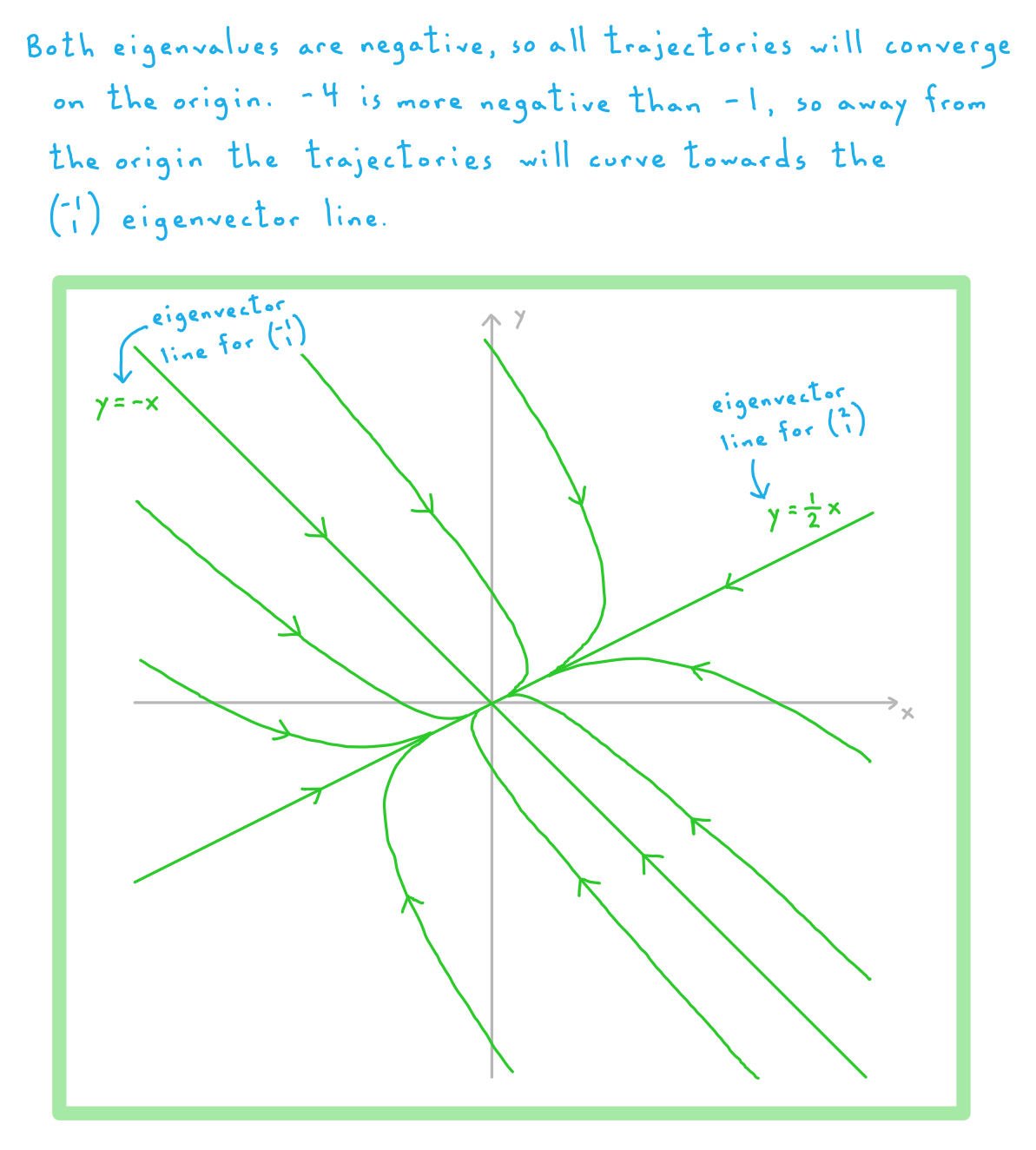
Equilibrium Points
What is an equilibrium point?
- For a system of coupled differential equations, an equilibrium point is a point
%3C%2Fmo%3E%3C%2Fmath%3E--%3E%3Cdefs%3E%3Cstyle%20type%3D%22text%2Fcss%22%3E%40font-face%7Bfont-family%3A'math1f7177163c833dff4b38fc8d287'%3Bsrc%3Aurl(data%3Afont%2Ftruetype%3Bcharset%3Dutf-8%3Bbase64%2CAAEAAAAMAIAAAwBAT1MvMi7iBBMAAADMAAAATmNtYXDEvmKUAAABHAAAADRjdnQgDVUNBwAAAVAAAAA6Z2x5ZoPi2VsAAAGMAAAAUmhlYWQQC2qxAAAB4AAAADZoaGVhCGsXSAAAAhgAAAAkaG10eE2rRkcAAAI8AAAACGxvY2EAHTwYAAACRAAAAAxtYXhwBT0FPgAAAlAAAAAgbmFtZaBxlY4AAAJwAAABn3Bvc3QB9wD6AAAEEAAAACBwcmVwa1uragAABDAAAAAUAAADSwGQAAUAAAQABAAAAAAABAAEAAAAAAAAAQEAAAAAAAAAAAAAAAAAAAAAAAAAAAAAAAAAAAAAACAgICAAAAAg1UADev96AAAD6ACWAAAAAAACAAEAAQAAABQAAwABAAAAFAAEACAAAAAEAAQAAQAAACz%2F%2FwAAACz%2F%2F%2F%2FVAAEAAAAAAAABVAMsAIABAABWACoCWAIeAQ4BLAIsAFoBgAKAAKAA1ACAAAAAAAAAACsAVQCAAKsA1QEAASsABwAAAAIAVQAAAwADqwADAAcAADMRIRElIREhVQKr%2FasCAP4AA6v8VVUDAAABAFX%2FZADVAIAACgAAMzUzFRQGByc%2BATdVgC8vGx4eAYB6PVEUKQ40MQAAAAEAAAABAADVeM5BXw889QADBAD%2F%2F%2F%2F%2F1joTc%2F%2F%2F%2F%2F%2FWOhNzAAD%2FIASAA6sAAAAKAAIAAQAAAAAAAQAAA%2Bj%2FagAAF3AAAP%2B2BIAAAQAAAAAAAAAAAAAAAAAAAAIDUgBVATMAVQAAAAAAAAAoAAAAUgABAAAAAgBeAAUAAAAAAAIAgAQAAAAAAAQAAN4AAAAAAAAAFQECAAAAAAAAAAEAEgAAAAAAAAAAAAIADgASAAAAAAAAAAMAMAAgAAAAAAAAAAQAEgBQAAAAAAAAAAUAFgBiAAAAAAAAAAYACQB4AAAAAAAAAAgAHACBAAEAAAAAAAEAEgAAAAEAAAAAAAIADgASAAEAAAAAAAMAMAAgAAEAAAAAAAQAEgBQAAEAAAAAAAUAFgBiAAEAAAAAAAYACQB4AAEAAAAAAAgAHACBAAMAAQQJAAEAEgAAAAMAAQQJAAIADgASAAMAAQQJAAMAMAAgAAMAAQQJAAQAEgBQAAMAAQQJAAUAFgBiAAMAAQQJAAYACQB4AAMAAQQJAAgAHACBAE0AYQB0AGgAIABGAG8AbgB0AFIAZQBnAHUAbABhAHIATQBhAHQAaABzACAARgBvAHIAIABNAG8AcgBlACAATQBhAHQAaAAgAEYAbwBuAHQATQBhAHQAaAAgAEYAbwBuAHQAVgBlAHIAcwBpAG8AbgAgADEALgAwTWF0aF9Gb250AE0AYQB0AGgAcwAgAEYAbwByACAATQBvAHIAZQAAAwAAAAAAAAH0APoAAAAAAAAAAAAAAAAAAAAAAAAAALkHEQAAjYUYALIAAAAVFBOxAAE%2F)format('truetype')%3Bfont-weight%3Anormal%3Bfont-style%3Anormal%3B%7D%40font-face%7Bfont-family%3A'round_brackets18549f92a457f2409'%3Bsrc%3Aurl(data%3Afont%2Ftruetype%3Bcharset%3Dutf-8%3Bbase64%2CAAEAAAAMAIAAAwBAT1MvMjwHLFQAAADMAAAATmNtYXDf7xCrAAABHAAAADxjdnQgBAkDLgAAAVgAAAASZ2x5ZmAOz2cAAAFsAAABJGhlYWQOKih8AAACkAAAADZoaGVhCvgVwgAAAsgAAAAkaG10eCA6AAIAAALsAAAADGxvY2EAAARLAAAC%2BAAAABBtYXhwBIgEWQAAAwgAAAAgbmFtZXHR30MAAAMoAAACOXBvc3QDogHPAAAFZAAAACBwcmVwupWEAAAABYQAAAAHAAAGcgGQAAUAAAgACAAAAAAACAAIAAAAAAAAAQIAAAAAAAAAAAAAAAAAAAAAAAAAAAAAAAAAAAAAACAgICAAAAAo8AMGe%2F57AAAHPgGyAAAAAAACAAEAAQAAABQAAwABAAAAFAAEACgAAAAGAAQAAQACACgAKf%2F%2FAAAAKAAp%2F%2F%2F%2F2f%2FZAAEAAAAAAAAAAAFUAFYBAAAsAKgDgAAyAAcAAAACAAAAKgDVA1UAAwAHAAA1MxEjEyMRM9XVq4CAKgMr%2FQAC1QABAAD%2B0AIgBtAACQBNGAGwChCwA9SwAxCwAtSwChCwBdSwBRCwANSwAxCwBzywAhCwCDwAsAoQsAPUsAMQsAfUsAoQsAXUsAoQsADUsAMQsAI8sAcQsAg8MTAREAEzABEQASMAAZCQ%2FnABkJD%2BcALQ%2FZD%2BcAGQAnACcAGQ%2FnAAAQAA%2FtACIAbQAAkATRgBsAoQsAPUsAMQsALUsAoQsAXUsAUQsADUsAMQsAc8sAIQsAg8ALAKELAD1LADELAH1LAKELAF1LAKELAA1LADELACPLAHELAIPDEwARABIwAREAEzAAIg%2FnCQAZD%2BcJABkALQ%2FZD%2BcAGQAnACcAGQ%2FnAAAQAAAAEAAPW2NYFfDzz1AAMIAP%2F%2F%2F%2F%2FVre7u%2F%2F%2F%2F%2F9Wt7u4AAP7QA7cG0AAAAAoAAgABAAAAAAABAAAHPv5OAAAXcAAA%2F%2F4DtwABAAAAAAAAAAAAAAAAAAAAAwDVAAACIAAAAiAAAAAAAAAAAAAkAAAAowAAASQAAQAAAAMACgACAAAAAAACAIAEAAAAAAAEAABNAAAAAAAAABUBAgAAAAAAAAABAD4AAAAAAAAAAAACAA4APgAAAAAAAAADAFwATAAAAAAAAAAEAD4AqAAAAAAAAAAFABYA5gAAAAAAAAAGAB8A%2FAAAAAAAAAAIABwBGwABAAAAAAABAD4AAAABAAAAAAACAA4APgABAAAAAAADAFwATAABAAAAAAAEAD4AqAABAAAAAAAFABYA5gABAAAAAAAGAB8A%2FAABAAAAAAAIABwBGwADAAEECQABAD4AAAADAAEECQACAA4APgADAAEECQADAFwATAADAAEECQAEAD4AqAADAAEECQAFABYA5gADAAEECQAGAB8A%2FAADAAEECQAIABwBGwBSAG8AdQBuAGQAIABiAHIAYQBjAGsAZQB0AHMAIAB3AGkAdABoACAAYQBzAGMAZQBuAHQAIAAxADgANQA0AFIAZQBnAHUAbABhAHIATQBhAHQAaABzACAARgBvAHIAIABNAG8AcgBlACAAUgBvAHUAbgBkACAAYgByAGEAYwBrAGUAdABzACAAdwBpAHQAaAAgAGEAcwBjAGUAbgB0ACAAMQA4ADUANABSAG8AdQBuAGQAIABiAHIAYQBjAGsAZQB0AHMAIAB3AGkAdABoACAAYQBzAGMAZQBuAHQAIAAxADgANQA0AFYAZQByAHMAaQBvAG4AIAAyAC4AMFJvdW5kX2JyYWNrZXRzX3dpdGhfYXNjZW50XzE4NTQATQBhAHQAaABzACAARgBvAHIAIABNAG8AcgBlAAAAAAMAAAAAAAADnwHPAAAAAAAAAAAAAAAAAAAAAAAAAAC5B%2F8AAY2FAA%3D%3D)format('truetype')%3Bfont-weight%3Anormal%3Bfont-style%3Anormal%3B%7D%3C%2Fstyle%3E%3C%2Fdefs%3E%3Ctext%20font-family%3D%22round_brackets18549f92a457f2409%22%20font-size%3D%2218%22%20text-anchor%3D%22middle%22%20x%3D%223.5%22%20y%3D%2216%22%3E(%3C%2Ftext%3E%3Ctext%20font-family%3D%22Times%20New%20Roman%22%20font-size%3D%2218%22%20font-style%3D%22italic%22%20text-anchor%3D%22middle%22%20x%3D%2210.5%22%20y%3D%2216%22%3Ex%3C%2Ftext%3E%3Ctext%20font-family%3D%22math1f7177163c833dff4b38fc8d287%22%20font-size%3D%2216%22%20text-anchor%3D%22middle%22%20x%3D%2218.5%22%20y%3D%2216%22%3E%2C%3C%2Ftext%3E%3Ctext%20font-family%3D%22Times%20New%20Roman%22%20font-size%3D%2218%22%20font-style%3D%22italic%22%20text-anchor%3D%22middle%22%20x%3D%2229.5%22%20y%3D%2216%22%3Ey%3C%2Ftext%3E%3Ctext%20font-family%3D%22round_brackets18549f92a457f2409%22%20font-size%3D%2218%22%20text-anchor%3D%22middle%22%20x%3D%2237.5%22%20y%3D%2216%22%3E)%3C%2Ftext%3E%3C%2Fsvg%3E) at which both
at which both format('truetype')%3Bfont-weight%3Anormal%3Bfont-style%3Anormal%3B%7D%3C%2Fstyle%3E%3C%2Fdefs%3E%3Cline%20stroke%3D%22%23000000%22%20stroke-linecap%3D%22square%22%20stroke-width%3D%221%22%20x1%3D%222.5%22%20x2%3D%2225.5%22%20y1%3D%2223.5%22%20y2%3D%2223.5%22%2F%3E%3Ctext%20font-family%3D%22Times%20New%20Roman%22%20font-size%3D%2218%22%20text-anchor%3D%22middle%22%20x%3D%229.5%22%20y%3D%2216%22%3Ed%3C%2Ftext%3E%3Ctext%20font-family%3D%22Times%20New%20Roman%22%20font-size%3D%2218%22%20font-style%3D%22italic%22%20text-anchor%3D%22middle%22%20x%3D%2218.5%22%20y%3D%2216%22%3Ex%3C%2Ftext%3E%3Ctext%20font-family%3D%22Times%20New%20Roman%22%20font-size%3D%2218%22%20text-anchor%3D%22middle%22%20x%3D%2211.5%22%20y%3D%2241%22%3Ed%3C%2Ftext%3E%3Ctext%20font-family%3D%22Times%20New%20Roman%22%20font-size%3D%2218%22%20font-style%3D%22italic%22%20text-anchor%3D%22middle%22%20x%3D%2218.5%22%20y%3D%2241%22%3Et%3C%2Ftext%3E%3Ctext%20font-family%3D%22math17f39f8317fbdb1988ef4c628eb%22%20font-size%3D%2216%22%20text-anchor%3D%22middle%22%20x%3D%2236.5%22%20y%3D%2230%22%3E%3D%3C%2Ftext%3E%3Ctext%20font-family%3D%22Times%20New%20Roman%22%20font-size%3D%2218%22%20text-anchor%3D%22middle%22%20x%3D%2249.5%22%20y%3D%2230%22%3E0%3C%2Ftext%3E%3C%2Fsvg%3E) and
and format('truetype')%3Bfont-weight%3Anormal%3Bfont-style%3Anormal%3B%7D%3C%2Fstyle%3E%3C%2Fdefs%3E%3Cline%20stroke%3D%22%23000000%22%20stroke-linecap%3D%22square%22%20stroke-width%3D%221%22%20x1%3D%222.5%22%20x2%3D%2225.5%22%20y1%3D%2223.5%22%20y2%3D%2223.5%22%2F%3E%3Ctext%20font-family%3D%22Times%20New%20Roman%22%20font-size%3D%2218%22%20text-anchor%3D%22middle%22%20x%3D%229.5%22%20y%3D%2216%22%3Ed%3C%2Ftext%3E%3Ctext%20font-family%3D%22Times%20New%20Roman%22%20font-size%3D%2218%22%20font-style%3D%22italic%22%20text-anchor%3D%22middle%22%20x%3D%2218.5%22%20y%3D%2216%22%3Ey%3C%2Ftext%3E%3Ctext%20font-family%3D%22Times%20New%20Roman%22%20font-size%3D%2218%22%20text-anchor%3D%22middle%22%20x%3D%2211.5%22%20y%3D%2241%22%3Ed%3C%2Ftext%3E%3Ctext%20font-family%3D%22Times%20New%20Roman%22%20font-size%3D%2218%22%20font-style%3D%22italic%22%20text-anchor%3D%22middle%22%20x%3D%2218.5%22%20y%3D%2241%22%3Et%3C%2Ftext%3E%3Ctext%20font-family%3D%22math17f39f8317fbdb1988ef4c628eb%22%20font-size%3D%2216%22%20text-anchor%3D%22middle%22%20x%3D%2236.5%22%20y%3D%2230%22%3E%3D%3C%2Ftext%3E%3Ctext%20font-family%3D%22Times%20New%20Roman%22%20font-size%3D%2218%22%20text-anchor%3D%22middle%22%20x%3D%2249.5%22%20y%3D%2230%22%3E0%3C%2Ftext%3E%3C%2Fsvg%3E)
- Because both derivatives are zero, the rates of change of both and are zero
- This means that and will not change, and therefore that if the system is ever at the point then it will remain at that point forever
- An equilibrium point can be stable or unstable
- An equilibrium point is stable if for all points close to the equilibrium point the solution trajectories move back towards the equilibrium point
- This means that if the system is perturbed away from the equilibrium point, it will tend to move back towards the state of equilibrium
- If an equilibrium point is not stable, then it is unstable
- If a system is perturbed away from an unstable equilibrium point, it will tend to continue moving further and further away from the state of equilibrium
- For a system that can be represented in the matrix form
format('truetype')%3Bfont-weight%3Anormal%3Bfont-style%3Anormal%3B%7D%3C%2Fstyle%3E%3C%2Fdefs%3E%3Ctext%20font-family%3D%22math1dd165a6c6b5bc8158c57065d13%22%20font-size%3D%2212%22%20text-anchor%3D%22middle%22%20x%3D%225.5%22%20y%3D%227%22%3E.%3C%2Ftext%3E%3Ctext%20font-family%3D%22Times%20New%20Roman%22%20font-size%3D%2218%22%20font-style%3D%22italic%22%20font-weight%3D%22bold%22%20text-anchor%3D%22middle%22%20x%3D%225.5%22%20y%3D%2218%22%3Ex%3C%2Ftext%3E%3Ctext%20font-family%3D%22math1dd165a6c6b5bc8158c57065d13%22%20font-size%3D%2216%22%20text-anchor%3D%22middle%22%20x%3D%2219.5%22%20y%3D%2218%22%3E%3D%3C%2Ftext%3E%3Ctext%20font-family%3D%22Times%20New%20Roman%22%20font-size%3D%2218%22%20font-style%3D%22italic%22%20font-weight%3D%22bold%22%20text-anchor%3D%22middle%22%20x%3D%2236.5%22%20y%3D%2218%22%3EM%3C%2Ftext%3E%3Ctext%20font-family%3D%22Times%20New%20Roman%22%20font-size%3D%2218%22%20font-style%3D%22italic%22%20font-weight%3D%22bold%22%20text-anchor%3D%22middle%22%20x%3D%2250.5%22%20y%3D%2218%22%3Ex%3C%2Ftext%3E%3C%2Fsvg%3E) , where , , and , the origin
, where , , and , the origin %3C%2Fmo%3E%3C%2Fmath%3E--%3E%3Cdefs%3E%3Cstyle%20type%3D%22text%2Fcss%22%3E%40font-face%7Bfont-family%3A'math1f7177163c833dff4b38fc8d287'%3Bsrc%3Aurl(data%3Afont%2Ftruetype%3Bcharset%3Dutf-8%3Bbase64%2CAAEAAAAMAIAAAwBAT1MvMi7iBBMAAADMAAAATmNtYXDEvmKUAAABHAAAADRjdnQgDVUNBwAAAVAAAAA6Z2x5ZoPi2VsAAAGMAAAAUmhlYWQQC2qxAAAB4AAAADZoaGVhCGsXSAAAAhgAAAAkaG10eE2rRkcAAAI8AAAACGxvY2EAHTwYAAACRAAAAAxtYXhwBT0FPgAAAlAAAAAgbmFtZaBxlY4AAAJwAAABn3Bvc3QB9wD6AAAEEAAAACBwcmVwa1uragAABDAAAAAUAAADSwGQAAUAAAQABAAAAAAABAAEAAAAAAAAAQEAAAAAAAAAAAAAAAAAAAAAAAAAAAAAAAAAAAAAACAgICAAAAAg1UADev96AAAD6ACWAAAAAAACAAEAAQAAABQAAwABAAAAFAAEACAAAAAEAAQAAQAAACz%2F%2FwAAACz%2F%2F%2F%2FVAAEAAAAAAAABVAMsAIABAABWACoCWAIeAQ4BLAIsAFoBgAKAAKAA1ACAAAAAAAAAACsAVQCAAKsA1QEAASsABwAAAAIAVQAAAwADqwADAAcAADMRIRElIREhVQKr%2FasCAP4AA6v8VVUDAAABAFX%2FZADVAIAACgAAMzUzFRQGByc%2BATdVgC8vGx4eAYB6PVEUKQ40MQAAAAEAAAABAADVeM5BXw889QADBAD%2F%2F%2F%2F%2F1joTc%2F%2F%2F%2F%2F%2FWOhNzAAD%2FIASAA6sAAAAKAAIAAQAAAAAAAQAAA%2Bj%2FagAAF3AAAP%2B2BIAAAQAAAAAAAAAAAAAAAAAAAAIDUgBVATMAVQAAAAAAAAAoAAAAUgABAAAAAgBeAAUAAAAAAAIAgAQAAAAAAAQAAN4AAAAAAAAAFQECAAAAAAAAAAEAEgAAAAAAAAAAAAIADgASAAAAAAAAAAMAMAAgAAAAAAAAAAQAEgBQAAAAAAAAAAUAFgBiAAAAAAAAAAYACQB4AAAAAAAAAAgAHACBAAEAAAAAAAEAEgAAAAEAAAAAAAIADgASAAEAAAAAAAMAMAAgAAEAAAAAAAQAEgBQAAEAAAAAAAUAFgBiAAEAAAAAAAYACQB4AAEAAAAAAAgAHACBAAMAAQQJAAEAEgAAAAMAAQQJAAIADgASAAMAAQQJAAMAMAAgAAMAAQQJAAQAEgBQAAMAAQQJAAUAFgBiAAMAAQQJAAYACQB4AAMAAQQJAAgAHACBAE0AYQB0AGgAIABGAG8AbgB0AFIAZQBnAHUAbABhAHIATQBhAHQAaABzACAARgBvAHIAIABNAG8AcgBlACAATQBhAHQAaAAgAEYAbwBuAHQATQBhAHQAaAAgAEYAbwBuAHQAVgBlAHIAcwBpAG8AbgAgADEALgAwTWF0aF9Gb250AE0AYQB0AGgAcwAgAEYAbwByACAATQBvAHIAZQAAAwAAAAAAAAH0APoAAAAAAAAAAAAAAAAAAAAAAAAAALkHEQAAjYUYALIAAAAVFBOxAAE%2F)format('truetype')%3Bfont-weight%3Anormal%3Bfont-style%3Anormal%3B%7D%40font-face%7Bfont-family%3A'round_brackets18549f92a457f2409'%3Bsrc%3Aurl(data%3Afont%2Ftruetype%3Bcharset%3Dutf-8%3Bbase64%2CAAEAAAAMAIAAAwBAT1MvMjwHLFQAAADMAAAATmNtYXDf7xCrAAABHAAAADxjdnQgBAkDLgAAAVgAAAASZ2x5ZmAOz2cAAAFsAAABJGhlYWQOKih8AAACkAAAADZoaGVhCvgVwgAAAsgAAAAkaG10eCA6AAIAAALsAAAADGxvY2EAAARLAAAC%2BAAAABBtYXhwBIgEWQAAAwgAAAAgbmFtZXHR30MAAAMoAAACOXBvc3QDogHPAAAFZAAAACBwcmVwupWEAAAABYQAAAAHAAAGcgGQAAUAAAgACAAAAAAACAAIAAAAAAAAAQIAAAAAAAAAAAAAAAAAAAAAAAAAAAAAAAAAAAAAACAgICAAAAAo8AMGe%2F57AAAHPgGyAAAAAAACAAEAAQAAABQAAwABAAAAFAAEACgAAAAGAAQAAQACACgAKf%2F%2FAAAAKAAp%2F%2F%2F%2F2f%2FZAAEAAAAAAAAAAAFUAFYBAAAsAKgDgAAyAAcAAAACAAAAKgDVA1UAAwAHAAA1MxEjEyMRM9XVq4CAKgMr%2FQAC1QABAAD%2B0AIgBtAACQBNGAGwChCwA9SwAxCwAtSwChCwBdSwBRCwANSwAxCwBzywAhCwCDwAsAoQsAPUsAMQsAfUsAoQsAXUsAoQsADUsAMQsAI8sAcQsAg8MTAREAEzABEQASMAAZCQ%2FnABkJD%2BcALQ%2FZD%2BcAGQAnACcAGQ%2FnAAAQAA%2FtACIAbQAAkATRgBsAoQsAPUsAMQsALUsAoQsAXUsAUQsADUsAMQsAc8sAIQsAg8ALAKELAD1LADELAH1LAKELAF1LAKELAA1LADELACPLAHELAIPDEwARABIwAREAEzAAIg%2FnCQAZD%2BcJABkALQ%2FZD%2BcAGQAnACcAGQ%2FnAAAQAAAAEAAPW2NYFfDzz1AAMIAP%2F%2F%2F%2F%2FVre7u%2F%2F%2F%2F%2F9Wt7u4AAP7QA7cG0AAAAAoAAgABAAAAAAABAAAHPv5OAAAXcAAA%2F%2F4DtwABAAAAAAAAAAAAAAAAAAAAAwDVAAACIAAAAiAAAAAAAAAAAAAkAAAAowAAASQAAQAAAAMACgACAAAAAAACAIAEAAAAAAAEAABNAAAAAAAAABUBAgAAAAAAAAABAD4AAAAAAAAAAAACAA4APgAAAAAAAAADAFwATAAAAAAAAAAEAD4AqAAAAAAAAAAFABYA5gAAAAAAAAAGAB8A%2FAAAAAAAAAAIABwBGwABAAAAAAABAD4AAAABAAAAAAACAA4APgABAAAAAAADAFwATAABAAAAAAAEAD4AqAABAAAAAAAFABYA5gABAAAAAAAGAB8A%2FAABAAAAAAAIABwBGwADAAEECQABAD4AAAADAAEECQACAA4APgADAAEECQADAFwATAADAAEECQAEAD4AqAADAAEECQAFABYA5gADAAEECQAGAB8A%2FAADAAEECQAIABwBGwBSAG8AdQBuAGQAIABiAHIAYQBjAGsAZQB0AHMAIAB3AGkAdABoACAAYQBzAGMAZQBuAHQAIAAxADgANQA0AFIAZQBnAHUAbABhAHIATQBhAHQAaABzACAARgBvAHIAIABNAG8AcgBlACAAUgBvAHUAbgBkACAAYgByAGEAYwBrAGUAdABzACAAdwBpAHQAaAAgAGEAcwBjAGUAbgB0ACAAMQA4ADUANABSAG8AdQBuAGQAIABiAHIAYQBjAGsAZQB0AHMAIAB3AGkAdABoACAAYQBzAGMAZQBuAHQAIAAxADgANQA0AFYAZQByAHMAaQBvAG4AIAAyAC4AMFJvdW5kX2JyYWNrZXRzX3dpdGhfYXNjZW50XzE4NTQATQBhAHQAaABzACAARgBvAHIAIABNAG8AcgBlAAAAAAMAAAAAAAADnwHPAAAAAAAAAAAAAAAAAAAAAAAAAAC5B%2F8AAY2FAA%3D%3D)format('truetype')%3Bfont-weight%3Anormal%3Bfont-style%3Anormal%3B%7D%3C%2Fstyle%3E%3C%2Fdefs%3E%3Ctext%20font-family%3D%22round_brackets18549f92a457f2409%22%20font-size%3D%2218%22%20text-anchor%3D%22middle%22%20x%3D%223.5%22%20y%3D%2216%22%3E(%3C%2Ftext%3E%3Ctext%20font-family%3D%22Times%20New%20Roman%22%20font-size%3D%2218%22%20text-anchor%3D%22middle%22%20x%3D%2210.5%22%20y%3D%2216%22%3E0%3C%2Ftext%3E%3Ctext%20font-family%3D%22math1f7177163c833dff4b38fc8d287%22%20font-size%3D%2216%22%20text-anchor%3D%22middle%22%20x%3D%2217.5%22%20y%3D%2216%22%3E%2C%3C%2Ftext%3E%3Ctext%20font-family%3D%22Times%20New%20Roman%22%20font-size%3D%2218%22%20text-anchor%3D%22middle%22%20x%3D%2228.5%22%20y%3D%2216%22%3E0%3C%2Ftext%3E%3Ctext%20font-family%3D%22round_brackets18549f92a457f2409%22%20font-size%3D%2218%22%20text-anchor%3D%22middle%22%20x%3D%2235.5%22%20y%3D%2216%22%3E)%3C%2Ftext%3E%3C%2Fsvg%3E) is always an equilibrium point
is always an equilibrium point - Considering the nature of the phase portrait for a particular system will tell us what sort of equilibrium point the origin is
- If both eigenvalues of the matrix are real and negative, then the origin is a stable equilibrium point
- This sort of equilibrium point is sometimes known as a sink
- If both eigenvalues of the matrix are real and positive, then the origin is an unstable equilibrium point
- This sort of equilibrium point is sometimes known as a source
- If both eigenvalues of the matrix are real, with one positive and one negative, then the origin is an unstable equilibrium point
- This sort of equilibrium point is known as a saddle point (you will be expected to identify saddle points if they occur in an AI HL exam question)
- If both eigenvalues of the matrix are imaginary, then the origin is an unstable equilibrium point
- Recall that for all points other than the origin, the solution trajectories here all ‘orbit’ around the origin along circular or elliptical paths
- If both eigenvalues of the matrix are complex with a negative real part, then the origin is an stable equilibrium point
- All solution trajectories here spiral in towards the origin
- If both eigenvalues of the matrix are complex with a positive real part, then the origin is an unstable equilibrium point
- All solution trajectories here spiral away from the origin
Worked Example
format('truetype')%3Bfont-weight%3Anormal%3Bfont-style%3Anormal%3B%7D%3C%2Fstyle%3E%3C%2Fdefs%3E%3Cline%20stroke%3D%22%23000000%22%20stroke-linecap%3D%22square%22%20stroke-width%3D%221%22%20x1%3D%222.5%22%20x2%3D%2225.5%22%20y1%3D%2223.5%22%20y2%3D%2223.5%22%2F%3E%3Ctext%20font-family%3D%22Times%20New%20Roman%22%20font-size%3D%2218%22%20text-anchor%3D%22middle%22%20x%3D%229.5%22%20y%3D%2216%22%3Ed%3C%2Ftext%3E%3Ctext%20font-family%3D%22Times%20New%20Roman%22%20font-size%3D%2218%22%20font-style%3D%22italic%22%20text-anchor%3D%22middle%22%20x%3D%2218.5%22%20y%3D%2216%22%3Ex%3C%2Ftext%3E%3Ctext%20font-family%3D%22Times%20New%20Roman%22%20font-size%3D%2218%22%20text-anchor%3D%22middle%22%20x%3D%2211.5%22%20y%3D%2241%22%3Ed%3C%2Ftext%3E%3Ctext%20font-family%3D%22Times%20New%20Roman%22%20font-size%3D%2218%22%20font-style%3D%22italic%22%20text-anchor%3D%22middle%22%20x%3D%2218.5%22%20y%3D%2241%22%3Et%3C%2Ftext%3E%3Ctext%20font-family%3D%22math190bc3972c7934354efb2af01e7%22%20font-size%3D%2216%22%20text-anchor%3D%22middle%22%20x%3D%2236.5%22%20y%3D%2230%22%3E%3D%3C%2Ftext%3E%3Ctext%20font-family%3D%22Times%20New%20Roman%22%20font-size%3D%2218%22%20text-anchor%3D%22middle%22%20x%3D%2249.5%22%20y%3D%2230%22%3E2%3C%2Ftext%3E%3Ctext%20font-family%3D%22Times%20New%20Roman%22%20font-size%3D%2218%22%20font-style%3D%22italic%22%20text-anchor%3D%22middle%22%20x%3D%2258.5%22%20y%3D%2230%22%3Ex%3C%2Ftext%3E%3Ctext%20font-family%3D%22math190bc3972c7934354efb2af01e7%22%20font-size%3D%2216%22%20text-anchor%3D%22middle%22%20x%3D%2272.5%22%20y%3D%2230%22%3E%26%23x2212%3B%3C%2Ftext%3E%3Ctext%20font-family%3D%22Times%20New%20Roman%22%20font-size%3D%2218%22%20text-anchor%3D%22middle%22%20x%3D%2285.5%22%20y%3D%2230%22%3E3%3C%2Ftext%3E%3Ctext%20font-family%3D%22Times%20New%20Roman%22%20font-size%3D%2218%22%20font-style%3D%22italic%22%20text-anchor%3D%22middle%22%20x%3D%2294.5%22%20y%3D%2230%22%3Ey%3C%2Ftext%3E%3Ctext%20font-family%3D%22math190bc3972c7934354efb2af01e7%22%20font-size%3D%2216%22%20text-anchor%3D%22middle%22%20x%3D%22108.5%22%20y%3D%2230%22%3E%2B%3C%2Ftext%3E%3Ctext%20font-family%3D%22Times%20New%20Roman%22%20font-size%3D%2218%22%20text-anchor%3D%22middle%22%20x%3D%22121.5%22%20y%3D%2230%22%3E6%3C%2Ftext%3E%3Cline%20stroke%3D%22%23000000%22%20stroke-linecap%3D%22square%22%20stroke-width%3D%221%22%20x1%3D%222.5%22%20x2%3D%2225.5%22%20y1%3D%2274.5%22%20y2%3D%2274.5%22%2F%3E%3Ctext%20font-family%3D%22Times%20New%20Roman%22%20font-size%3D%2218%22%20text-anchor%3D%22middle%22%20x%3D%229.5%22%20y%3D%2267%22%3Ed%3C%2Ftext%3E%3Ctext%20font-family%3D%22Times%20New%20Roman%22%20font-size%3D%2218%22%20font-style%3D%22italic%22%20text-anchor%3D%22middle%22%20x%3D%2218.5%22%20y%3D%2267%22%3Ey%3C%2Ftext%3E%3Ctext%20font-family%3D%22Times%20New%20Roman%22%20font-size%3D%2218%22%20text-anchor%3D%22middle%22%20x%3D%2211.5%22%20y%3D%2292%22%3Ed%3C%2Ftext%3E%3Ctext%20font-family%3D%22Times%20New%20Roman%22%20font-size%3D%2218%22%20font-style%3D%22italic%22%20text-anchor%3D%22middle%22%20x%3D%2218.5%22%20y%3D%2292%22%3Et%3C%2Ftext%3E%3Ctext%20font-family%3D%22math190bc3972c7934354efb2af01e7%22%20font-size%3D%2216%22%20text-anchor%3D%22middle%22%20x%3D%2236.5%22%20y%3D%2281%22%3E%3D%3C%2Ftext%3E%3Ctext%20font-family%3D%22Times%20New%20Roman%22%20font-size%3D%2218%22%20font-style%3D%22italic%22%20text-anchor%3D%22middle%22%20x%3D%2249.5%22%20y%3D%2281%22%3Ex%3C%2Ftext%3E%3Ctext%20font-family%3D%22math190bc3972c7934354efb2af01e7%22%20font-size%3D%2216%22%20text-anchor%3D%22middle%22%20x%3D%2263.5%22%20y%3D%2281%22%3E%2B%3C%2Ftext%3E%3Ctext%20font-family%3D%22Times%20New%20Roman%22%20font-size%3D%2218%22%20font-style%3D%22italic%22%20text-anchor%3D%22middle%22%20x%3D%2276.5%22%20y%3D%2281%22%3Ey%3C%2Ftext%3E%3Ctext%20font-family%3D%22math190bc3972c7934354efb2af01e7%22%20font-size%3D%2216%22%20text-anchor%3D%22middle%22%20x%3D%2290.5%22%20y%3D%2281%22%3E%26%23x2212%3B%3C%2Ftext%3E%3Ctext%20font-family%3D%22Times%20New%20Roman%22%20font-size%3D%2218%22%20text-anchor%3D%22middle%22%20x%3D%22103.5%22%20y%3D%2281%22%3E7%3C%2Ftext%3E%3C%2Fsvg%3E)
Show that %3C%2Fmo%3E%3C%2Fmath%3E--%3E%3Cdefs%3E%3Cstyle%20type%3D%22text%2Fcss%22%3E%40font-face%7Bfont-family%3A'math1f7177163c833dff4b38fc8d287'%3Bsrc%3Aurl(data%3Afont%2Ftruetype%3Bcharset%3Dutf-8%3Bbase64%2CAAEAAAAMAIAAAwBAT1MvMi7iBBMAAADMAAAATmNtYXDEvmKUAAABHAAAADRjdnQgDVUNBwAAAVAAAAA6Z2x5ZoPi2VsAAAGMAAAAUmhlYWQQC2qxAAAB4AAAADZoaGVhCGsXSAAAAhgAAAAkaG10eE2rRkcAAAI8AAAACGxvY2EAHTwYAAACRAAAAAxtYXhwBT0FPgAAAlAAAAAgbmFtZaBxlY4AAAJwAAABn3Bvc3QB9wD6AAAEEAAAACBwcmVwa1uragAABDAAAAAUAAADSwGQAAUAAAQABAAAAAAABAAEAAAAAAAAAQEAAAAAAAAAAAAAAAAAAAAAAAAAAAAAAAAAAAAAACAgICAAAAAg1UADev96AAAD6ACWAAAAAAACAAEAAQAAABQAAwABAAAAFAAEACAAAAAEAAQAAQAAACz%2F%2FwAAACz%2F%2F%2F%2FVAAEAAAAAAAABVAMsAIABAABWACoCWAIeAQ4BLAIsAFoBgAKAAKAA1ACAAAAAAAAAACsAVQCAAKsA1QEAASsABwAAAAIAVQAAAwADqwADAAcAADMRIRElIREhVQKr%2FasCAP4AA6v8VVUDAAABAFX%2FZADVAIAACgAAMzUzFRQGByc%2BATdVgC8vGx4eAYB6PVEUKQ40MQAAAAEAAAABAADVeM5BXw889QADBAD%2F%2F%2F%2F%2F1joTc%2F%2F%2F%2F%2F%2FWOhNzAAD%2FIASAA6sAAAAKAAIAAQAAAAAAAQAAA%2Bj%2FagAAF3AAAP%2B2BIAAAQAAAAAAAAAAAAAAAAAAAAIDUgBVATMAVQAAAAAAAAAoAAAAUgABAAAAAgBeAAUAAAAAAAIAgAQAAAAAAAQAAN4AAAAAAAAAFQECAAAAAAAAAAEAEgAAAAAAAAAAAAIADgASAAAAAAAAAAMAMAAgAAAAAAAAAAQAEgBQAAAAAAAAAAUAFgBiAAAAAAAAAAYACQB4AAAAAAAAAAgAHACBAAEAAAAAAAEAEgAAAAEAAAAAAAIADgASAAEAAAAAAAMAMAAgAAEAAAAAAAQAEgBQAAEAAAAAAAUAFgBiAAEAAAAAAAYACQB4AAEAAAAAAAgAHACBAAMAAQQJAAEAEgAAAAMAAQQJAAIADgASAAMAAQQJAAMAMAAgAAMAAQQJAAQAEgBQAAMAAQQJAAUAFgBiAAMAAQQJAAYACQB4AAMAAQQJAAgAHACBAE0AYQB0AGgAIABGAG8AbgB0AFIAZQBnAHUAbABhAHIATQBhAHQAaABzACAARgBvAHIAIABNAG8AcgBlACAATQBhAHQAaAAgAEYAbwBuAHQATQBhAHQAaAAgAEYAbwBuAHQAVgBlAHIAcwBpAG8AbgAgADEALgAwTWF0aF9Gb250AE0AYQB0AGgAcwAgAEYAbwByACAATQBvAHIAZQAAAwAAAAAAAAH0APoAAAAAAAAAAAAAAAAAAAAAAAAAALkHEQAAjYUYALIAAAAVFBOxAAE%2F)format('truetype')%3Bfont-weight%3Anormal%3Bfont-style%3Anormal%3B%7D%40font-face%7Bfont-family%3A'round_brackets18549f92a457f2409'%3Bsrc%3Aurl(data%3Afont%2Ftruetype%3Bcharset%3Dutf-8%3Bbase64%2CAAEAAAAMAIAAAwBAT1MvMjwHLFQAAADMAAAATmNtYXDf7xCrAAABHAAAADxjdnQgBAkDLgAAAVgAAAASZ2x5ZmAOz2cAAAFsAAABJGhlYWQOKih8AAACkAAAADZoaGVhCvgVwgAAAsgAAAAkaG10eCA6AAIAAALsAAAADGxvY2EAAARLAAAC%2BAAAABBtYXhwBIgEWQAAAwgAAAAgbmFtZXHR30MAAAMoAAACOXBvc3QDogHPAAAFZAAAACBwcmVwupWEAAAABYQAAAAHAAAGcgGQAAUAAAgACAAAAAAACAAIAAAAAAAAAQIAAAAAAAAAAAAAAAAAAAAAAAAAAAAAAAAAAAAAACAgICAAAAAo8AMGe%2F57AAAHPgGyAAAAAAACAAEAAQAAABQAAwABAAAAFAAEACgAAAAGAAQAAQACACgAKf%2F%2FAAAAKAAp%2F%2F%2F%2F2f%2FZAAEAAAAAAAAAAAFUAFYBAAAsAKgDgAAyAAcAAAACAAAAKgDVA1UAAwAHAAA1MxEjEyMRM9XVq4CAKgMr%2FQAC1QABAAD%2B0AIgBtAACQBNGAGwChCwA9SwAxCwAtSwChCwBdSwBRCwANSwAxCwBzywAhCwCDwAsAoQsAPUsAMQsAfUsAoQsAXUsAoQsADUsAMQsAI8sAcQsAg8MTAREAEzABEQASMAAZCQ%2FnABkJD%2BcALQ%2FZD%2BcAGQAnACcAGQ%2FnAAAQAA%2FtACIAbQAAkATRgBsAoQsAPUsAMQsALUsAoQsAXUsAUQsADUsAMQsAc8sAIQsAg8ALAKELAD1LADELAH1LAKELAF1LAKELAA1LADELACPLAHELAIPDEwARABIwAREAEzAAIg%2FnCQAZD%2BcJABkALQ%2FZD%2BcAGQAnACcAGQ%2FnAAAQAAAAEAAPW2NYFfDzz1AAMIAP%2F%2F%2F%2F%2FVre7u%2F%2F%2F%2F%2F9Wt7u4AAP7QA7cG0AAAAAoAAgABAAAAAAABAAAHPv5OAAAXcAAA%2F%2F4DtwABAAAAAAAAAAAAAAAAAAAAAwDVAAACIAAAAiAAAAAAAAAAAAAkAAAAowAAASQAAQAAAAMACgACAAAAAAACAIAEAAAAAAAEAABNAAAAAAAAABUBAgAAAAAAAAABAD4AAAAAAAAAAAACAA4APgAAAAAAAAADAFwATAAAAAAAAAAEAD4AqAAAAAAAAAAFABYA5gAAAAAAAAAGAB8A%2FAAAAAAAAAAIABwBGwABAAAAAAABAD4AAAABAAAAAAACAA4APgABAAAAAAADAFwATAABAAAAAAAEAD4AqAABAAAAAAAFABYA5gABAAAAAAAGAB8A%2FAABAAAAAAAIABwBGwADAAEECQABAD4AAAADAAEECQACAA4APgADAAEECQADAFwATAADAAEECQAEAD4AqAADAAEECQAFABYA5gADAAEECQAGAB8A%2FAADAAEECQAIABwBGwBSAG8AdQBuAGQAIABiAHIAYQBjAGsAZQB0AHMAIAB3AGkAdABoACAAYQBzAGMAZQBuAHQAIAAxADgANQA0AFIAZQBnAHUAbABhAHIATQBhAHQAaABzACAARgBvAHIAIABNAG8AcgBlACAAUgBvAHUAbgBkACAAYgByAGEAYwBrAGUAdABzACAAdwBpAHQAaAAgAGEAcwBjAGUAbgB0ACAAMQA4ADUANABSAG8AdQBuAGQAIABiAHIAYQBjAGsAZQB0AHMAIAB3AGkAdABoACAAYQBzAGMAZQBuAHQAIAAxADgANQA0AFYAZQByAHMAaQBvAG4AIAAyAC4AMFJvdW5kX2JyYWNrZXRzX3dpdGhfYXNjZW50XzE4NTQATQBhAHQAaABzACAARgBvAHIAIABNAG8AcgBlAAAAAAMAAAAAAAADnwHPAAAAAAAAAAAAAAAAAAAAAAAAAAC5B%2F8AAY2FAA%3D%3D)format('truetype')%3Bfont-weight%3Anormal%3Bfont-style%3Anormal%3B%7D%3C%2Fstyle%3E%3C%2Fdefs%3E%3Ctext%20font-family%3D%22round_brackets18549f92a457f2409%22%20font-size%3D%2218%22%20text-anchor%3D%22middle%22%20x%3D%223.5%22%20y%3D%2216%22%3E(%3C%2Ftext%3E%3Ctext%20font-family%3D%22Times%20New%20Roman%22%20font-size%3D%2218%22%20text-anchor%3D%22middle%22%20x%3D%2210.5%22%20y%3D%2216%22%3E3%3C%2Ftext%3E%3Ctext%20font-family%3D%22math1f7177163c833dff4b38fc8d287%22%20font-size%3D%2216%22%20text-anchor%3D%22middle%22%20x%3D%2217.5%22%20y%3D%2216%22%3E%2C%3C%2Ftext%3E%3Ctext%20font-family%3D%22Times%20New%20Roman%22%20font-size%3D%2218%22%20text-anchor%3D%22middle%22%20x%3D%2228.5%22%20y%3D%2216%22%3E4%3C%2Ftext%3E%3Ctext%20font-family%3D%22round_brackets18549f92a457f2409%22%20font-size%3D%2218%22%20text-anchor%3D%22middle%22%20x%3D%2235.5%22%20y%3D%2216%22%3E)%3C%2Ftext%3E%3C%2Fsvg%3E) is an equilibrium point for the system.
is an equilibrium point for the system.
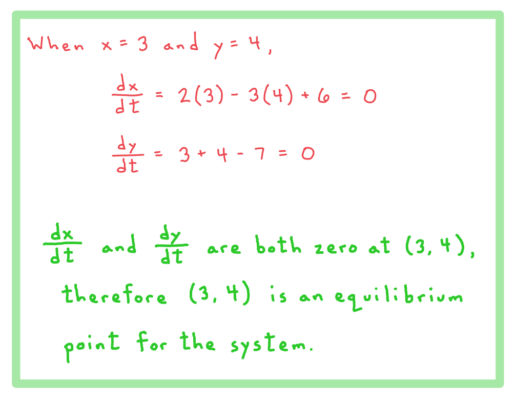
format('truetype')%3Bfont-weight%3Anormal%3Bfont-style%3Anormal%3B%7D%3C%2Fstyle%3E%3C%2Fdefs%3E%3Cline%20stroke%3D%22%23000000%22%20stroke-linecap%3D%22square%22%20stroke-width%3D%221%22%20x1%3D%222.5%22%20x2%3D%2225.5%22%20y1%3D%2223.5%22%20y2%3D%2223.5%22%2F%3E%3Ctext%20font-family%3D%22Times%20New%20Roman%22%20font-size%3D%2218%22%20text-anchor%3D%22middle%22%20x%3D%229.5%22%20y%3D%2216%22%3Ed%3C%2Ftext%3E%3Ctext%20font-family%3D%22Times%20New%20Roman%22%20font-size%3D%2218%22%20font-style%3D%22italic%22%20text-anchor%3D%22middle%22%20x%3D%2218.5%22%20y%3D%2216%22%3Ex%3C%2Ftext%3E%3Ctext%20font-family%3D%22Times%20New%20Roman%22%20font-size%3D%2218%22%20text-anchor%3D%22middle%22%20x%3D%2211.5%22%20y%3D%2241%22%3Ed%3C%2Ftext%3E%3Ctext%20font-family%3D%22Times%20New%20Roman%22%20font-size%3D%2218%22%20font-style%3D%22italic%22%20text-anchor%3D%22middle%22%20x%3D%2218.5%22%20y%3D%2241%22%3Et%3C%2Ftext%3E%3Ctext%20font-family%3D%22math1564b4c0e54101ac57a0cb68c16%22%20font-size%3D%2216%22%20text-anchor%3D%22middle%22%20x%3D%2236.5%22%20y%3D%2230%22%3E%3D%3C%2Ftext%3E%3Ctext%20font-family%3D%22Times%20New%20Roman%22%20font-size%3D%2218%22%20font-style%3D%22italic%22%20text-anchor%3D%22middle%22%20x%3D%2249.5%22%20y%3D%2230%22%3Ex%3C%2Ftext%3E%3Ctext%20font-family%3D%22math1564b4c0e54101ac57a0cb68c16%22%20font-size%3D%2216%22%20text-anchor%3D%22middle%22%20x%3D%2263.5%22%20y%3D%2230%22%3E%2B%3C%2Ftext%3E%3Ctext%20font-family%3D%22Times%20New%20Roman%22%20font-size%3D%2218%22%20text-anchor%3D%22middle%22%20x%3D%2276.5%22%20y%3D%2230%22%3E3%3C%2Ftext%3E%3Ctext%20font-family%3D%22Times%20New%20Roman%22%20font-size%3D%2218%22%20font-style%3D%22italic%22%20text-anchor%3D%22middle%22%20x%3D%2285.5%22%20y%3D%2230%22%3Ey%3C%2Ftext%3E%3Cline%20stroke%3D%22%23000000%22%20stroke-linecap%3D%22square%22%20stroke-width%3D%221%22%20x1%3D%222.5%22%20x2%3D%2225.5%22%20y1%3D%2274.5%22%20y2%3D%2274.5%22%2F%3E%3Ctext%20font-family%3D%22Times%20New%20Roman%22%20font-size%3D%2218%22%20text-anchor%3D%22middle%22%20x%3D%229.5%22%20y%3D%2267%22%3Ed%3C%2Ftext%3E%3Ctext%20font-family%3D%22Times%20New%20Roman%22%20font-size%3D%2218%22%20font-style%3D%22italic%22%20text-anchor%3D%22middle%22%20x%3D%2218.5%22%20y%3D%2267%22%3Ey%3C%2Ftext%3E%3Ctext%20font-family%3D%22Times%20New%20Roman%22%20font-size%3D%2218%22%20text-anchor%3D%22middle%22%20x%3D%2211.5%22%20y%3D%2292%22%3Ed%3C%2Ftext%3E%3Ctext%20font-family%3D%22Times%20New%20Roman%22%20font-size%3D%2218%22%20font-style%3D%22italic%22%20text-anchor%3D%22middle%22%20x%3D%2218.5%22%20y%3D%2292%22%3Et%3C%2Ftext%3E%3Ctext%20font-family%3D%22math1564b4c0e54101ac57a0cb68c16%22%20font-size%3D%2216%22%20text-anchor%3D%22middle%22%20x%3D%2236.5%22%20y%3D%2281%22%3E%3D%3C%2Ftext%3E%3Ctext%20font-family%3D%22Times%20New%20Roman%22%20font-size%3D%2218%22%20text-anchor%3D%22middle%22%20x%3D%2249.5%22%20y%3D%2281%22%3E2%3C%2Ftext%3E%3Ctext%20font-family%3D%22Times%20New%20Roman%22%20font-size%3D%2218%22%20font-style%3D%22italic%22%20text-anchor%3D%22middle%22%20x%3D%2258.5%22%20y%3D%2281%22%3Ex%3C%2Ftext%3E%3Ctext%20font-family%3D%22math1564b4c0e54101ac57a0cb68c16%22%20font-size%3D%2216%22%20text-anchor%3D%22middle%22%20x%3D%2272.5%22%20y%3D%2281%22%3E%2B%3C%2Ftext%3E%3Ctext%20font-family%3D%22Times%20New%20Roman%22%20font-size%3D%2218%22%20text-anchor%3D%22middle%22%20x%3D%2285.5%22%20y%3D%2281%22%3E2%3C%2Ftext%3E%3Ctext%20font-family%3D%22Times%20New%20Roman%22%20font-size%3D%2218%22%20font-style%3D%22italic%22%20text-anchor%3D%22middle%22%20x%3D%2294.5%22%20y%3D%2281%22%3Ey%3C%2Ftext%3E%3C%2Fsvg%3E)
Given that  and are the eigenvalues of the matrix
 format('truetype')%3Bfont-weight%3Anormal%3Bfont-style%3Anormal%3B%7D%40font-face%7Bfont-family%3A'bracketse552f5417ff4680c6b50499'%3Bsrc%3Aurl(data%3Afont%2Ftruetype%3Bcharset%3Dutf-8%3Bbase64%2CAAEAAAAMAIAAAwBAT1MvMi7RIisAAADMAAAATmNtYXBi7uzYAAABHAAAAExjdnQgBAkDLgAAAWgAAAASZ2x5Zo64f%2BkAAAF8AAABSWhlYWQLniGcAAACyAAAADZoaGVhBK4XLAAAAwAAAAAkaG10eCWq%2F90AAAMkAAAAFGxvY2EAABknAAADOAAAABhtYXhwBJIESAAAA1AAAAAgbmFtZRAA8I4AAANwAAAB3nBvc3QBwwDgAAAFUAAAACBwcmVwupWEAAAABXAAAAAHAAACggGQAAUAAAQABAAAAAAABAAEAAAAAAAAAQEAAAAAAAAAAAAAAAAAAAAAAAAAAAAAAAAAAAAAACAgICAAAAAg9AMEAAAAAAADgAAAAAAAAAACAAEAAQAAABQAAwABAAAAFAAEADgAAAAKAAgAAgACI5sjnSOeI6D%2F%2FwAAI5sjnSOeI6D%2F%2F9xm3GXcZdxkAAEAAAAAAAAAAAAAAAABVABWAQAALACoA4AAMgAHAAAAAgAAACoA1QNVAAMABwAANTMRIxMjETPV1auAgCoDK%2F0AAtUAAQAAAAABgAOAAAUAJBgBsAAvsAPFsQEC%2FbADELEEBP0AsQAAP7ABPLEEBj%2BwAzwwMTEzEAEjAFUBKyv%2BqwH8AYT%2BqgABAAAAAAGAA4AABQAmGAGwAC6wA8WxBQL9sAMQsQIE%2FQB8sQAGPxiwBTyxAwb2sAI8MDEREgEzABMBAVQr%2FtMCA4D91v6qAYQB%2FAAB%2F6wAAAEsA4AABQAnGAGwAC%2BwBzywA8WxAQL9sAMQsQQE%2FQCxAAA%2FsAE8sQQGP7ADPDAxISMSATMAASxVAf7UKwFVAfwBhP6rAAH%2FrAAAASwDgAAFACkYAbABL7AHPLAExbEAAv2wBBCxAwT9AHyxAQY%2FsAA8GLEEAD%2BwAzwwMRMzEAEjANdV%2FqsrASsDgP3V%2FqsBhgAAAAABAAAAAQAAeuTcpl8PPPUAAwQA%2F%2F%2F%2F%2F9Wt7o7%2F%2F%2F%2F%2F1a3ujv%2BsAAABgAOAAAAACgACAAEAAAAAAAEAAAOAAAAAABdw%2F6z%2FrAGAAAEAAAAAAAAAAAAAAAAAAAAFANUAAAEsAAABLAAAASz%2FrAEs%2F6wAAAAAAAAAJAAAAGgAAACzAAAA%2FQAAAUkAAQAAAAUACAACAAAAAAACAIAEAAAAAAAEAAA%2BAAAAAAAAABUBAgAAAAAAAAABACQAAAAAAAAAAAACAA4AJAAAAAAAAAADAEIAMgAAAAAAAAAEACQAdAAAAAAAAAAFABYAmAAAAAAAAAAGABIArgAAAAAAAAAIABwAwAABAAAAAAABACQAAAABAAAAAAACAA4AJAABAAAAAAADAEIAMgABAAAAAAAEACQAdAABAAAAAAAFABYAmAABAAAAAAAGABIArgABAAAAAAAIABwAwAADAAEECQABACQAAAADAAEECQACAA4AJAADAAEECQADAEIAMgADAAEECQAEACQAdAADAAEECQAFABYAmAADAAEECQAGABIArgADAAEECQAIABwAwABCAHIAYQBjAGsAZQB0AHMAIABmAHUAbABsACAAcwBpAHoAZQBSAGUAZwB1AGwAYQByAE0AYQB0AGgAcwAgAEYAbwByACAATQBvAHIAZQAgAEIAcgBhAGMAawBlAHQAcwAgAGYAdQBsAGwAIABzAGkAegBlAEIAcgBhAGMAawBlAHQAcwAgAGYAdQBsAGwAIABzAGkAegBlAFYAZQByAHMAaQBvAG4AIAAyAC4AMEJyYWNrZXRzX2Z1bGxfc2l6ZQBNAGEAdABoAHMAIABGAG8AcgAgAE0AbwByAGUAAAADAAAAAAAAAcAA4AAAAAAAAAAAAAAAAAAAAAAAAAAAuQf%2FAAGNhQA%3D)format('truetype')%3Bfont-weight%3Anormal%3Bfont-style%3Anormal%3B%7D%3C%2Fstyle%3E%3C%2Fdefs%3E%3Ctext%20font-family%3D%22bracketse552f5417ff4680c6b50499%22%20font-size%3D%2218%22%20text-anchor%3D%22start%22%20x%3D%221.5%22%20y%3D%2218%22%3E%26%23x239B%3B%3C%2Ftext%3E%3Ctext%20font-family%3D%22brack_sm2882ad605b1e27be87c7468%22%20font-size%3D%2218%22%20text-anchor%3D%22start%22%20x%3D%221.5%22%20y%3D%2224%22%3E%26%23x239C%3B%3C%2Ftext%3E%3Ctext%20font-family%3D%22brack_sm2882ad605b1e27be87c7468%22%20font-size%3D%2218%22%20text-anchor%3D%22start%22%20x%3D%221.5%22%20y%3D%2230%22%3E%26%23x239C%3B%3C%2Ftext%3E%3Ctext%20font-family%3D%22brack_sm2882ad605b1e27be87c7468%22%20font-size%3D%2218%22%20text-anchor%3D%22start%22%20x%3D%221.5%22%20y%3D%2236%22%3E%26%23x239C%3B%3C%2Ftext%3E%3Ctext%20font-family%3D%22bracketse552f5417ff4680c6b50499%22%20font-size%3D%2218%22%20text-anchor%3D%22start%22%20x%3D%221.5%22%20y%3D%2252%22%3E%26%23x239D%3B%3C%2Ftext%3E%3Ctext%20font-family%3D%22bracketse552f5417ff4680c6b50499%22%20font-size%3D%2218%22%20text-anchor%3D%22start%22%20x%3D%2242.5%22%20y%3D%2218%22%3E%26%23x239E%3B%3C%2Ftext%3E%3Ctext%20font-family%3D%22brack_sm2882ad605b1e27be87c7468%22%20font-size%3D%2218%22%20text-anchor%3D%22start%22%20x%3D%2242.5%22%20y%3D%2224%22%3E%26%23x239F%3B%3C%2Ftext%3E%3Ctext%20font-family%3D%22brack_sm2882ad605b1e27be87c7468%22%20font-size%3D%2218%22%20text-anchor%3D%22start%22%20x%3D%2242.5%22%20y%3D%2230%22%3E%26%23x239F%3B%3C%2Ftext%3E%3Ctext%20font-family%3D%22brack_sm2882ad605b1e27be87c7468%22%20font-size%3D%2218%22%20text-anchor%3D%22start%22%20x%3D%2242.5%22%20y%3D%2236%22%3E%26%23x239F%3B%3C%2Ftext%3E%3Ctext%20font-family%3D%22bracketse552f5417ff4680c6b50499%22%20font-size%3D%2218%22%20text-anchor%3D%22start%22%20x%3D%2242.5%22%20y%3D%2252%22%3E%26%23x23A0%3B%3C%2Ftext%3E%3Ctext%20font-family%3D%22Times%20New%20Roman%22%20font-size%3D%2218%22%20text-anchor%3D%22middle%22%20x%3D%2215.5%22%20y%3D%2219%22%3E1%3C%2Ftext%3E%3Ctext%20font-family%3D%22Times%20New%20Roman%22%20font-size%3D%2218%22%20text-anchor%3D%22middle%22%20x%3D%2232.5%22%20y%3D%2219%22%3E3%3C%2Ftext%3E%3Ctext%20font-family%3D%22Times%20New%20Roman%22%20font-size%3D%2218%22%20text-anchor%3D%22middle%22%20x%3D%2215.5%22%20y%3D%2245%22%3E2%3C%2Ftext%3E%3Ctext%20font-family%3D%22Times%20New%20Roman%22%20font-size%3D%2218%22%20text-anchor%3D%22middle%22%20x%3D%2232.5%22%20y%3D%2245%22%3E2%3C%2Ftext%3E%3C%2Fsvg%3E) , with corresponding eigenvectors and
, with corresponding eigenvectors and format('truetype')%3Bfont-weight%3Anormal%3Bfont-style%3Anormal%3B%7D%40font-face%7Bfont-family%3A'brack_sm2882ad605b1e27be87c7468'%3Bsrc%3Aurl(data%3Afont%2Ftruetype%3Bcharset%3Dutf-8%3Bbase64%2CAAEAAAAMAIAAAwBAT1MvMi7PH4UAAADMAAAATmNtYXA3kjw6AAABHAAAADxjdnQgAQYDiAAAAVgAAAASZ2x5ZkyYQ7YAAAFsAAAAkWhlYWQLyR8fAAACAAAAADZoaGVhAq0XCAAAAjgAAAAkaG10eDEjA%2FUAAAJcAAAADGxvY2EAAEKZAAACaAAAABBtYXhwBJsEcQAAAngAAAAgbmFtZW7QvZAAAAKYAAAB5XBvc3QArQBVAAAEgAAAACBwcmVwu5WEAAAABKAAAAAHAAACDAGQAAUAAAQABAAAAAAABAAEAAAAAAAAAQEAAAAAAAAAAAAAAAAAAAAAAAAAAAAAAAAAAAAAACAgICAAAAAg9AMD%2FP%2F8AAABVAABAAAAAAACAAEAAQAAABQAAwABAAAAFAAEACgAAAAGAAQAAQACI5wjn%2F%2F%2FAAAjnCOf%2F%2F%2FcZdxjAAEAAAAAAAAAAAFUAFQBAAArAIwAgACoAAcAAAACAAAAAADVAQEAAwAHAAAxMxEjFyM1M9XVq4CAAQHWqwABAAAAAABVAVgAAwAfGAGwAy%2BwADyxAgL1sAE8ALEDAD%2BwAjx8sQAG9bABPBEzESNVVQFY%2FqgAAQDXAAABLAFUAAMAIBgBsAUvsAE8sAI8sQAC9bADPACwAy%2BwAjyxAAH1sAE8EzMRI9dVVQFU%2FqwAAAAAAQAAAAEAAIsesexfDzz1AAMEAP%2F%2F%2F%2F%2FVre5k%2F%2F%2F%2F%2F9Wt7mT%2FgP%2F%2FAdYBWAAAAAoAAgABAAAAAAABAAABVP%2F%2FAAAXcP%2BA%2F4AB1gABAAAAAAAAAAAAAAAAAAAAAwDVAAABLAAAASwA1wAAAAAAAAAhAAAAWAAAAJEAAQAAAAMACgACAAAAAAACAIAEAAAAAAAEAABlAAAAAAAAABUBAgAAAAAAAAABACYAAAAAAAAAAAACAA4AJgAAAAAAAAADAEQANAAAAAAAAAAEACYAeAAAAAAAAAAFABYAngAAAAAAAAAGABMAtAAAAAAAAAAIABwAxwABAAAAAAABACYAAAABAAAAAAACAA4AJgABAAAAAAADAEQANAABAAAAAAAEACYAeAABAAAAAAAFABYAngABAAAAAAAGABMAtAABAAAAAAAIABwAxwADAAEECQABACYAAAADAAEECQACAA4AJgADAAEECQADAEQANAADAAEECQAEACYAeAADAAEECQAFABYAngADAAEECQAGABMAtAADAAEECQAIABwAxwBCAHIAYQBjAGsAZQB0AHMAIABzAG0AYQBsAGwAIABzAGkAegBlAFIAZQBnAHUAbABhAHIATQBhAHQAaABzACAARgBvAHIAIABNAG8AcgBlACAAQgByAGEAYwBrAGUAdABzACAAcwBtAGEAbABsACAAcwBpAHoAZQBCAHIAYQBjAGsAZQB0AHMAIABzAG0AYQBsAGwAIABzAGkAegBlAFYAZQByAHMAaQBvAG4AIAAyAC4AMEJyYWNrZXRzX3NtYWxsX3NpemUATQBhAHQAaABzACAARgBvAHIAIABNAG8AcgBlAAAAAAMAAAAAAAAAqgBVAAAAAAAAAAAAAAAAAAAAAAAAAAC5B%2F8AAo2FAA%3D%3D)format('truetype')%3Bfont-weight%3Anormal%3Bfont-style%3Anormal%3B%7D%40font-face%7Bfont-family%3A'bracketse552f5417ff4680c6b50499'%3Bsrc%3Aurl(data%3Afont%2Ftruetype%3Bcharset%3Dutf-8%3Bbase64%2CAAEAAAAMAIAAAwBAT1MvMi7RIisAAADMAAAATmNtYXBi7uzYAAABHAAAAExjdnQgBAkDLgAAAWgAAAASZ2x5Zo64f%2BkAAAF8AAABSWhlYWQLniGcAAACyAAAADZoaGVhBK4XLAAAAwAAAAAkaG10eCWq%2F90AAAMkAAAAFGxvY2EAABknAAADOAAAABhtYXhwBJIESAAAA1AAAAAgbmFtZRAA8I4AAANwAAAB3nBvc3QBwwDgAAAFUAAAACBwcmVwupWEAAAABXAAAAAHAAACggGQAAUAAAQABAAAAAAABAAEAAAAAAAAAQEAAAAAAAAAAAAAAAAAAAAAAAAAAAAAAAAAAAAAACAgICAAAAAg9AMEAAAAAAADgAAAAAAAAAACAAEAAQAAABQAAwABAAAAFAAEADgAAAAKAAgAAgACI5sjnSOeI6D%2F%2FwAAI5sjnSOeI6D%2F%2F9xm3GXcZdxkAAEAAAAAAAAAAAAAAAABVABWAQAALACoA4AAMgAHAAAAAgAAACoA1QNVAAMABwAANTMRIxMjETPV1auAgCoDK%2F0AAtUAAQAAAAABgAOAAAUAJBgBsAAvsAPFsQEC%2FbADELEEBP0AsQAAP7ABPLEEBj%2BwAzwwMTEzEAEjAFUBKyv%2BqwH8AYT%2BqgABAAAAAAGAA4AABQAmGAGwAC6wA8WxBQL9sAMQsQIE%2FQB8sQAGPxiwBTyxAwb2sAI8MDEREgEzABMBAVQr%2FtMCA4D91v6qAYQB%2FAAB%2F6wAAAEsA4AABQAnGAGwAC%2BwBzywA8WxAQL9sAMQsQQE%2FQCxAAA%2FsAE8sQQGP7ADPDAxISMSATMAASxVAf7UKwFVAfwBhP6rAAH%2FrAAAASwDgAAFACkYAbABL7AHPLAExbEAAv2wBBCxAwT9AHyxAQY%2FsAA8GLEEAD%2BwAzwwMRMzEAEjANdV%2FqsrASsDgP3V%2FqsBhgAAAAABAAAAAQAAeuTcpl8PPPUAAwQA%2F%2F%2F%2F%2F9Wt7o7%2F%2F%2F%2F%2F1a3ujv%2BsAAABgAOAAAAACgACAAEAAAAAAAEAAAOAAAAAABdw%2F6z%2FrAGAAAEAAAAAAAAAAAAAAAAAAAAFANUAAAEsAAABLAAAASz%2FrAEs%2F6wAAAAAAAAAJAAAAGgAAACzAAAA%2FQAAAUkAAQAAAAUACAACAAAAAAACAIAEAAAAAAAEAAA%2BAAAAAAAAABUBAgAAAAAAAAABACQAAAAAAAAAAAACAA4AJAAAAAAAAAADAEIAMgAAAAAAAAAEACQAdAAAAAAAAAAFABYAmAAAAAAAAAAGABIArgAAAAAAAAAIABwAwAABAAAAAAABACQAAAABAAAAAAACAA4AJAABAAAAAAADAEIAMgABAAAAAAAEACQAdAABAAAAAAAFABYAmAABAAAAAAAGABIArgABAAAAAAAIABwAwAADAAEECQABACQAAAADAAEECQACAA4AJAADAAEECQADAEIAMgADAAEECQAEACQAdAADAAEECQAFABYAmAADAAEECQAGABIArgADAAEECQAIABwAwABCAHIAYQBjAGsAZQB0AHMAIABmAHUAbABsACAAcwBpAHoAZQBSAGUAZwB1AGwAYQByAE0AYQB0AGgAcwAgAEYAbwByACAATQBvAHIAZQAgAEIAcgBhAGMAawBlAHQAcwAgAGYAdQBsAGwAIABzAGkAegBlAEIAcgBhAGMAawBlAHQAcwAgAGYAdQBsAGwAIABzAGkAegBlAFYAZQByAHMAaQBvAG4AIAAyAC4AMEJyYWNrZXRzX2Z1bGxfc2l6ZQBNAGEAdABoAHMAIABGAG8AcgAgAE0AbwByAGUAAAADAAAAAAAAAcAA4AAAAAAAAAAAAAAAAAAAAAAAAAAAuQf%2FAAGNhQA%3D)format('truetype')%3Bfont-weight%3Anormal%3Bfont-style%3Anormal%3B%7D%3C%2Fstyle%3E%3C%2Fdefs%3E%3Ctext%20font-family%3D%22bracketse552f5417ff4680c6b50499%22%20font-size%3D%2218%22%20text-anchor%3D%22start%22%20x%3D%221.5%22%20y%3D%2218%22%3E%26%23x239B%3B%3C%2Ftext%3E%3Ctext%20font-family%3D%22brack_sm2882ad605b1e27be87c7468%22%20font-size%3D%2218%22%20text-anchor%3D%22start%22%20x%3D%221.5%22%20y%3D%2224%22%3E%26%23x239C%3B%3C%2Ftext%3E%3Ctext%20font-family%3D%22brack_sm2882ad605b1e27be87c7468%22%20font-size%3D%2218%22%20text-anchor%3D%22start%22%20x%3D%221.5%22%20y%3D%2230%22%3E%26%23x239C%3B%3C%2Ftext%3E%3Ctext%20font-family%3D%22brack_sm2882ad605b1e27be87c7468%22%20font-size%3D%2218%22%20text-anchor%3D%22start%22%20x%3D%221.5%22%20y%3D%2236%22%3E%26%23x239C%3B%3C%2Ftext%3E%3Ctext%20font-family%3D%22bracketse552f5417ff4680c6b50499%22%20font-size%3D%2218%22%20text-anchor%3D%22start%22%20x%3D%221.5%22%20y%3D%2252%22%3E%26%23x239D%3B%3C%2Ftext%3E%3Ctext%20font-family%3D%22bracketse552f5417ff4680c6b50499%22%20font-size%3D%2218%22%20text-anchor%3D%22start%22%20x%3D%2238.5%22%20y%3D%2218%22%3E%26%23x239E%3B%3C%2Ftext%3E%3Ctext%20font-family%3D%22brack_sm2882ad605b1e27be87c7468%22%20font-size%3D%2218%22%20text-anchor%3D%22start%22%20x%3D%2238.5%22%20y%3D%2224%22%3E%26%23x239F%3B%3C%2Ftext%3E%3Ctext%20font-family%3D%22brack_sm2882ad605b1e27be87c7468%22%20font-size%3D%2218%22%20text-anchor%3D%22start%22%20x%3D%2238.5%22%20y%3D%2230%22%3E%26%23x239F%3B%3C%2Ftext%3E%3Ctext%20font-family%3D%22brack_sm2882ad605b1e27be87c7468%22%20font-size%3D%2218%22%20text-anchor%3D%22start%22%20x%3D%2238.5%22%20y%3D%2236%22%3E%26%23x239F%3B%3C%2Ftext%3E%3Ctext%20font-family%3D%22bracketse552f5417ff4680c6b50499%22%20font-size%3D%2218%22%20text-anchor%3D%22start%22%20x%3D%2238.5%22%20y%3D%2252%22%3E%26%23x23A0%3B%3C%2Ftext%3E%3Ctext%20font-family%3D%22math1da40657c9fece7e48d30af42d3%22%20font-size%3D%2216%22%20text-anchor%3D%22middle%22%20x%3D%2217.5%22%20y%3D%2219%22%3E%26%23x2212%3B%3C%2Ftext%3E%3Ctext%20font-family%3D%22Times%20New%20Roman%22%20font-size%3D%2218%22%20text-anchor%3D%22middle%22%20x%3D%2228.5%22%20y%3D%2219%22%3E3%3C%2Ftext%3E%3Ctext%20font-family%3D%22Times%20New%20Roman%22%20font-size%3D%2218%22%20text-anchor%3D%22middle%22%20x%3D%2221.5%22%20y%3D%2245%22%3E2%3C%2Ftext%3E%3C%2Fsvg%3E) , determine the coordinates and nature of the equilibrium point for the system.
, determine the coordinates and nature of the equilibrium point for the system.
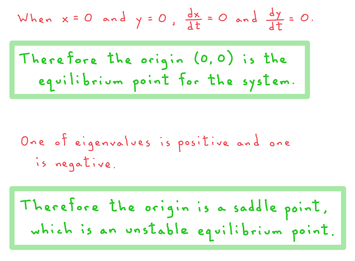
Sketching Solution Trajectories
How do I sketch a solution trajectory for a system of coupled differential equations?
- A phase portrait shows typical trajectories representing all the possible solutions to a system of coupled differential equations
- For a given set of initial conditions, however, the solution will only have one specific trajectory
- Sketching a particular solution trajectory will generally involve the following:
- Make sure you know what the ‘typical’ solutions for the system look like
- You don’t need to sketch a complete phase portrait unless asked, but you should know what the phase portrait for your system would look like
- If the phase portrait includes ‘eigenvector lines’, however, it is worth including these in your sketch to serve as guidelines
- Mark the starting point for your solution trajectory
- The coordinates of the starting point will be the and values when
format('truetype')%3Bfont-weight%3Anormal%3Bfont-style%3Anormal%3B%7D%3C%2Fstyle%3E%3C%2Fdefs%3E%3Ctext%20font-family%3D%22Times%20New%20Roman%22%20font-size%3D%2218%22%20font-style%3D%22italic%22%20text-anchor%3D%22middle%22%20x%3D%222.5%22%20y%3D%2216%22%3Et%3C%2Ftext%3E%3Ctext%20font-family%3D%22math17f39f8317fbdb1988ef4c628eb%22%20font-size%3D%2216%22%20text-anchor%3D%22middle%22%20x%3D%2214.5%22%20y%3D%2216%22%3E%3D%3C%2Ftext%3E%3Ctext%20font-family%3D%22Times%20New%20Roman%22%20font-size%3D%2218%22%20text-anchor%3D%22middle%22%20x%3D%2227.5%22%20y%3D%2216%22%3E0%3C%2Ftext%3E%3C%2Fsvg%3E)
- Usually these are given in the question as the initial conditions for the system
- Determine the initial direction of the solution trajectory
- To do this find the values of and when
- This will tell you the directions in which and are changing initially
- For example if
format('truetype')%3Bfont-weight%3Anormal%3Bfont-style%3Anormal%3B%7D%3C%2Fstyle%3E%3C%2Fdefs%3E%3Cline%20stroke%3D%22%23000000%22%20stroke-linecap%3D%22square%22%20stroke-width%3D%221%22%20x1%3D%222.5%22%20x2%3D%2225.5%22%20y1%3D%2223.5%22%20y2%3D%2223.5%22%2F%3E%3Ctext%20font-family%3D%22Times%20New%20Roman%22%20font-size%3D%2218%22%20text-anchor%3D%22middle%22%20x%3D%229.5%22%20y%3D%2216%22%3Ed%3C%2Ftext%3E%3Ctext%20font-family%3D%22Times%20New%20Roman%22%20font-size%3D%2218%22%20font-style%3D%22italic%22%20text-anchor%3D%22middle%22%20x%3D%2218.5%22%20y%3D%2216%22%3Ex%3C%2Ftext%3E%3Ctext%20font-family%3D%22Times%20New%20Roman%22%20font-size%3D%2218%22%20text-anchor%3D%22middle%22%20x%3D%2211.5%22%20y%3D%2241%22%3Ed%3C%2Ftext%3E%3Ctext%20font-family%3D%22Times%20New%20Roman%22%20font-size%3D%2218%22%20font-style%3D%22italic%22%20text-anchor%3D%22middle%22%20x%3D%2218.5%22%20y%3D%2241%22%3Et%3C%2Ftext%3E%3Ctext%20font-family%3D%22math143f4d31b04031e49f5eb18baba%22%20font-size%3D%2216%22%20text-anchor%3D%22middle%22%20x%3D%2236.5%22%20y%3D%2230%22%3E%3D%3C%2Ftext%3E%3Ctext%20font-family%3D%22math143f4d31b04031e49f5eb18baba%22%20font-size%3D%2216%22%20text-anchor%3D%22middle%22%20x%3D%2253.5%22%20y%3D%2230%22%3E%26%23x2212%3B%3C%2Ftext%3E%3Ctext%20font-family%3D%22Times%20New%20Roman%22%20font-size%3D%2218%22%20text-anchor%3D%22middle%22%20x%3D%2266.5%22%20y%3D%2230%22%3E2%3C%2Ftext%3E%3C%2Fsvg%3E) and
and format('truetype')%3Bfont-weight%3Anormal%3Bfont-style%3Anormal%3B%7D%3C%2Fstyle%3E%3C%2Fdefs%3E%3Cline%20stroke%3D%22%23000000%22%20stroke-linecap%3D%22square%22%20stroke-width%3D%221%22%20x1%3D%222.5%22%20x2%3D%2225.5%22%20y1%3D%2223.5%22%20y2%3D%2223.5%22%2F%3E%3Ctext%20font-family%3D%22Times%20New%20Roman%22%20font-size%3D%2218%22%20text-anchor%3D%22middle%22%20x%3D%229.5%22%20y%3D%2216%22%3Ed%3C%2Ftext%3E%3Ctext%20font-family%3D%22Times%20New%20Roman%22%20font-size%3D%2218%22%20font-style%3D%22italic%22%20text-anchor%3D%22middle%22%20x%3D%2218.5%22%20y%3D%2216%22%3Ey%3C%2Ftext%3E%3Ctext%20font-family%3D%22Times%20New%20Roman%22%20font-size%3D%2218%22%20text-anchor%3D%22middle%22%20x%3D%2211.5%22%20y%3D%2241%22%3Ed%3C%2Ftext%3E%3Ctext%20font-family%3D%22Times%20New%20Roman%22%20font-size%3D%2218%22%20font-style%3D%22italic%22%20text-anchor%3D%22middle%22%20x%3D%2218.5%22%20y%3D%2241%22%3Et%3C%2Ftext%3E%3Ctext%20font-family%3D%22math17f39f8317fbdb1988ef4c628eb%22%20font-size%3D%2216%22%20text-anchor%3D%22middle%22%20x%3D%2236.5%22%20y%3D%2230%22%3E%3D%3C%2Ftext%3E%3Ctext%20font-family%3D%22Times%20New%20Roman%22%20font-size%3D%2218%22%20text-anchor%3D%22middle%22%20x%3D%2249.5%22%20y%3D%2230%22%3E3%3C%2Ftext%3E%3C%2Fsvg%3E) when , then the trajectory from the starting point will initially be ‘to the left and up’, parallel to the vector
when , then the trajectory from the starting point will initially be ‘to the left and up’, parallel to the vector format('truetype')%3Bfont-weight%3Anormal%3Bfont-style%3Anormal%3B%7D%40font-face%7Bfont-family%3A'brack_sm2882ad605b1e27be87c7468'%3Bsrc%3Aurl(data%3Afont%2Ftruetype%3Bcharset%3Dutf-8%3Bbase64%2CAAEAAAAMAIAAAwBAT1MvMi7PH4UAAADMAAAATmNtYXA3kjw6AAABHAAAADxjdnQgAQYDiAAAAVgAAAASZ2x5ZkyYQ7YAAAFsAAAAkWhlYWQLyR8fAAACAAAAADZoaGVhAq0XCAAAAjgAAAAkaG10eDEjA%2FUAAAJcAAAADGxvY2EAAEKZAAACaAAAABBtYXhwBJsEcQAAAngAAAAgbmFtZW7QvZAAAAKYAAAB5XBvc3QArQBVAAAEgAAAACBwcmVwu5WEAAAABKAAAAAHAAACDAGQAAUAAAQABAAAAAAABAAEAAAAAAAAAQEAAAAAAAAAAAAAAAAAAAAAAAAAAAAAAAAAAAAAACAgICAAAAAg9AMD%2FP%2F8AAABVAABAAAAAAACAAEAAQAAABQAAwABAAAAFAAEACgAAAAGAAQAAQACI5wjn%2F%2F%2FAAAjnCOf%2F%2F%2FcZdxjAAEAAAAAAAAAAAFUAFQBAAArAIwAgACoAAcAAAACAAAAAADVAQEAAwAHAAAxMxEjFyM1M9XVq4CAAQHWqwABAAAAAABVAVgAAwAfGAGwAy%2BwADyxAgL1sAE8ALEDAD%2BwAjx8sQAG9bABPBEzESNVVQFY%2FqgAAQDXAAABLAFUAAMAIBgBsAUvsAE8sAI8sQAC9bADPACwAy%2BwAjyxAAH1sAE8EzMRI9dVVQFU%2FqwAAAAAAQAAAAEAAIsesexfDzz1AAMEAP%2F%2F%2F%2F%2FVre5k%2F%2F%2F%2F%2F9Wt7mT%2FgP%2F%2FAdYBWAAAAAoAAgABAAAAAAABAAABVP%2F%2FAAAXcP%2BA%2F4AB1gABAAAAAAAAAAAAAAAAAAAAAwDVAAABLAAAASwA1wAAAAAAAAAhAAAAWAAAAJEAAQAAAAMACgACAAAAAAACAIAEAAAAAAAEAABlAAAAAAAAABUBAgAAAAAAAAABACYAAAAAAAAAAAACAA4AJgAAAAAAAAADAEQANAAAAAAAAAAEACYAeAAAAAAAAAAFABYAngAAAAAAAAAGABMAtAAAAAAAAAAIABwAxwABAAAAAAABACYAAAABAAAAAAACAA4AJgABAAAAAAADAEQANAABAAAAAAAEACYAeAABAAAAAAAFABYAngABAAAAAAAGABMAtAABAAAAAAAIABwAxwADAAEECQABACYAAAADAAEECQACAA4AJgADAAEECQADAEQANAADAAEECQAEACYAeAADAAEECQAFABYAngADAAEECQAGABMAtAADAAEECQAIABwAxwBCAHIAYQBjAGsAZQB0AHMAIABzAG0AYQBsAGwAIABzAGkAegBlAFIAZQBnAHUAbABhAHIATQBhAHQAaABzACAARgBvAHIAIABNAG8AcgBlACAAQgByAGEAYwBrAGUAdABzACAAcwBtAGEAbABsACAAcwBpAHoAZQBCAHIAYQBjAGsAZQB0AHMAIABzAG0AYQBsAGwAIABzAGkAegBlAFYAZQByAHMAaQBvAG4AIAAyAC4AMEJyYWNrZXRzX3NtYWxsX3NpemUATQBhAHQAaABzACAARgBvAHIAIABNAG8AcgBlAAAAAAMAAAAAAAAAqgBVAAAAAAAAAAAAAAAAAAAAAAAAAAC5B%2F8AAo2FAA%3D%3D)format('truetype')%3Bfont-weight%3Anormal%3Bfont-style%3Anormal%3B%7D%40font-face%7Bfont-family%3A'bracketse552f5417ff4680c6b50499'%3Bsrc%3Aurl(data%3Afont%2Ftruetype%3Bcharset%3Dutf-8%3Bbase64%2CAAEAAAAMAIAAAwBAT1MvMi7RIisAAADMAAAATmNtYXBi7uzYAAABHAAAAExjdnQgBAkDLgAAAWgAAAASZ2x5Zo64f%2BkAAAF8AAABSWhlYWQLniGcAAACyAAAADZoaGVhBK4XLAAAAwAAAAAkaG10eCWq%2F90AAAMkAAAAFGxvY2EAABknAAADOAAAABhtYXhwBJIESAAAA1AAAAAgbmFtZRAA8I4AAANwAAAB3nBvc3QBwwDgAAAFUAAAACBwcmVwupWEAAAABXAAAAAHAAACggGQAAUAAAQABAAAAAAABAAEAAAAAAAAAQEAAAAAAAAAAAAAAAAAAAAAAAAAAAAAAAAAAAAAACAgICAAAAAg9AMEAAAAAAADgAAAAAAAAAACAAEAAQAAABQAAwABAAAAFAAEADgAAAAKAAgAAgACI5sjnSOeI6D%2F%2FwAAI5sjnSOeI6D%2F%2F9xm3GXcZdxkAAEAAAAAAAAAAAAAAAABVABWAQAALACoA4AAMgAHAAAAAgAAACoA1QNVAAMABwAANTMRIxMjETPV1auAgCoDK%2F0AAtUAAQAAAAABgAOAAAUAJBgBsAAvsAPFsQEC%2FbADELEEBP0AsQAAP7ABPLEEBj%2BwAzwwMTEzEAEjAFUBKyv%2BqwH8AYT%2BqgABAAAAAAGAA4AABQAmGAGwAC6wA8WxBQL9sAMQsQIE%2FQB8sQAGPxiwBTyxAwb2sAI8MDEREgEzABMBAVQr%2FtMCA4D91v6qAYQB%2FAAB%2F6wAAAEsA4AABQAnGAGwAC%2BwBzywA8WxAQL9sAMQsQQE%2FQCxAAA%2FsAE8sQQGP7ADPDAxISMSATMAASxVAf7UKwFVAfwBhP6rAAH%2FrAAAASwDgAAFACkYAbABL7AHPLAExbEAAv2wBBCxAwT9AHyxAQY%2FsAA8GLEEAD%2BwAzwwMRMzEAEjANdV%2FqsrASsDgP3V%2FqsBhgAAAAABAAAAAQAAeuTcpl8PPPUAAwQA%2F%2F%2F%2F%2F9Wt7o7%2F%2F%2F%2F%2F1a3ujv%2BsAAABgAOAAAAACgACAAEAAAAAAAEAAAOAAAAAABdw%2F6z%2FrAGAAAEAAAAAAAAAAAAAAAAAAAAFANUAAAEsAAABLAAAASz%2FrAEs%2F6wAAAAAAAAAJAAAAGgAAACzAAAA%2FQAAAUkAAQAAAAUACAACAAAAAAACAIAEAAAAAAAEAAA%2BAAAAAAAAABUBAgAAAAAAAAABACQAAAAAAAAAAAACAA4AJAAAAAAAAAADAEIAMgAAAAAAAAAEACQAdAAAAAAAAAAFABYAmAAAAAAAAAAGABIArgAAAAAAAAAIABwAwAABAAAAAAABACQAAAABAAAAAAACAA4AJAABAAAAAAADAEIAMgABAAAAAAAEACQAdAABAAAAAAAFABYAmAABAAAAAAAGABIArgABAAAAAAAIABwAwAADAAEECQABACQAAAADAAEECQACAA4AJAADAAEECQADAEIAMgADAAEECQAEACQAdAADAAEECQAFABYAmAADAAEECQAGABIArgADAAEECQAIABwAwABCAHIAYQBjAGsAZQB0AHMAIABmAHUAbABsACAAcwBpAHoAZQBSAGUAZwB1AGwAYQByAE0AYQB0AGgAcwAgAEYAbwByACAATQBvAHIAZQAgAEIAcgBhAGMAawBlAHQAcwAgAGYAdQBsAGwAIABzAGkAegBlAEIAcgBhAGMAawBlAHQAcwAgAGYAdQBsAGwAIABzAGkAegBlAFYAZQByAHMAaQBvAG4AIAAyAC4AMEJyYWNrZXRzX2Z1bGxfc2l6ZQBNAGEAdABoAHMAIABGAG8AcgAgAE0AbwByAGUAAAADAAAAAAAAAcAA4AAAAAAAAAAAAAAAAAAAAAAAAAAAuQf%2FAAGNhQA%3D)format('truetype')%3Bfont-weight%3Anormal%3Bfont-style%3Anormal%3B%7D%3C%2Fstyle%3E%3C%2Fdefs%3E%3Ctext%20font-family%3D%22bracketse552f5417ff4680c6b50499%22%20font-size%3D%2218%22%20text-anchor%3D%22start%22%20x%3D%221.5%22%20y%3D%2218%22%3E%26%23x239B%3B%3C%2Ftext%3E%3Ctext%20font-family%3D%22brack_sm2882ad605b1e27be87c7468%22%20font-size%3D%2218%22%20text-anchor%3D%22start%22%20x%3D%221.5%22%20y%3D%2224%22%3E%26%23x239C%3B%3C%2Ftext%3E%3Ctext%20font-family%3D%22brack_sm2882ad605b1e27be87c7468%22%20font-size%3D%2218%22%20text-anchor%3D%22start%22%20x%3D%221.5%22%20y%3D%2230%22%3E%26%23x239C%3B%3C%2Ftext%3E%3Ctext%20font-family%3D%22brack_sm2882ad605b1e27be87c7468%22%20font-size%3D%2218%22%20text-anchor%3D%22start%22%20x%3D%221.5%22%20y%3D%2236%22%3E%26%23x239C%3B%3C%2Ftext%3E%3Ctext%20font-family%3D%22bracketse552f5417ff4680c6b50499%22%20font-size%3D%2218%22%20text-anchor%3D%22start%22%20x%3D%221.5%22%20y%3D%2252%22%3E%26%23x239D%3B%3C%2Ftext%3E%3Ctext%20font-family%3D%22bracketse552f5417ff4680c6b50499%22%20font-size%3D%2218%22%20text-anchor%3D%22start%22%20x%3D%2238.5%22%20y%3D%2218%22%3E%26%23x239E%3B%3C%2Ftext%3E%3Ctext%20font-family%3D%22brack_sm2882ad605b1e27be87c7468%22%20font-size%3D%2218%22%20text-anchor%3D%22start%22%20x%3D%2238.5%22%20y%3D%2224%22%3E%26%23x239F%3B%3C%2Ftext%3E%3Ctext%20font-family%3D%22brack_sm2882ad605b1e27be87c7468%22%20font-size%3D%2218%22%20text-anchor%3D%22start%22%20x%3D%2238.5%22%20y%3D%2230%22%3E%26%23x239F%3B%3C%2Ftext%3E%3Ctext%20font-family%3D%22brack_sm2882ad605b1e27be87c7468%22%20font-size%3D%2218%22%20text-anchor%3D%22start%22%20x%3D%2238.5%22%20y%3D%2236%22%3E%26%23x239F%3B%3C%2Ftext%3E%3Ctext%20font-family%3D%22bracketse552f5417ff4680c6b50499%22%20font-size%3D%2218%22%20text-anchor%3D%22start%22%20x%3D%2238.5%22%20y%3D%2252%22%3E%26%23x23A0%3B%3C%2Ftext%3E%3Ctext%20font-family%3D%22math1da40657c9fece7e48d30af42d3%22%20font-size%3D%2216%22%20text-anchor%3D%22middle%22%20x%3D%2217.5%22%20y%3D%2219%22%3E%26%23x2212%3B%3C%2Ftext%3E%3Ctext%20font-family%3D%22Times%20New%20Roman%22%20font-size%3D%2218%22%20text-anchor%3D%22middle%22%20x%3D%2228.5%22%20y%3D%2219%22%3E2%3C%2Ftext%3E%3Ctext%20font-family%3D%22Times%20New%20Roman%22%20font-size%3D%2218%22%20text-anchor%3D%22middle%22%20x%3D%2221.5%22%20y%3D%2245%22%3E3%3C%2Ftext%3E%3C%2Fsvg%3E)
- Use the above considerations to create your sketch
- The trajectory should begin at the starting point (be sure to mark and label the starting point on your sketch!)
- It should move away from the starting point in the correct initial direction
- As it moves further away from the starting point, the trajectory should conform to the nature of a ‘typical solution’ for the system
Worked Example
Consider the system of coupled differential equations
format('truetype')%3Bfont-weight%3Anormal%3Bfont-style%3Anormal%3B%7D%3C%2Fstyle%3E%3C%2Fdefs%3E%3Cline%20stroke%3D%22%23000000%22%20stroke-linecap%3D%22square%22%20stroke-width%3D%221%22%20x1%3D%222.5%22%20x2%3D%2225.5%22%20y1%3D%2223.5%22%20y2%3D%2223.5%22%2F%3E%3Ctext%20font-family%3D%22Times%20New%20Roman%22%20font-size%3D%2218%22%20text-anchor%3D%22middle%22%20x%3D%229.5%22%20y%3D%2216%22%3Ed%3C%2Ftext%3E%3Ctext%20font-family%3D%22Times%20New%20Roman%22%20font-size%3D%2218%22%20font-style%3D%22italic%22%20text-anchor%3D%22middle%22%20x%3D%2218.5%22%20y%3D%2216%22%3Ex%3C%2Ftext%3E%3Ctext%20font-family%3D%22Times%20New%20Roman%22%20font-size%3D%2218%22%20text-anchor%3D%22middle%22%20x%3D%2211.5%22%20y%3D%2241%22%3Ed%3C%2Ftext%3E%3Ctext%20font-family%3D%22Times%20New%20Roman%22%20font-size%3D%2218%22%20font-style%3D%22italic%22%20text-anchor%3D%22middle%22%20x%3D%2218.5%22%20y%3D%2241%22%3Et%3C%2Ftext%3E%3Ctext%20font-family%3D%22math190bc3972c7934354efb2af01e7%22%20font-size%3D%2216%22%20text-anchor%3D%22middle%22%20x%3D%2236.5%22%20y%3D%2230%22%3E%3D%3C%2Ftext%3E%3Ctext%20font-family%3D%22Times%20New%20Roman%22%20font-size%3D%2218%22%20font-style%3D%22italic%22%20text-anchor%3D%22middle%22%20x%3D%2249.5%22%20y%3D%2230%22%3Ex%3C%2Ftext%3E%3Ctext%20font-family%3D%22math190bc3972c7934354efb2af01e7%22%20font-size%3D%2216%22%20text-anchor%3D%22middle%22%20x%3D%2263.5%22%20y%3D%2230%22%3E%26%23x2212%3B%3C%2Ftext%3E%3Ctext%20font-family%3D%22Times%20New%20Roman%22%20font-size%3D%2218%22%20text-anchor%3D%22middle%22%20x%3D%2276.5%22%20y%3D%2230%22%3E5%3C%2Ftext%3E%3Ctext%20font-family%3D%22Times%20New%20Roman%22%20font-size%3D%2218%22%20font-style%3D%22italic%22%20text-anchor%3D%22middle%22%20x%3D%2285.5%22%20y%3D%2230%22%3Ey%3C%2Ftext%3E%3Cline%20stroke%3D%22%23000000%22%20stroke-linecap%3D%22square%22%20stroke-width%3D%221%22%20x1%3D%222.5%22%20x2%3D%2225.5%22%20y1%3D%2274.5%22%20y2%3D%2274.5%22%2F%3E%3Ctext%20font-family%3D%22Times%20New%20Roman%22%20font-size%3D%2218%22%20text-anchor%3D%22middle%22%20x%3D%229.5%22%20y%3D%2267%22%3Ed%3C%2Ftext%3E%3Ctext%20font-family%3D%22Times%20New%20Roman%22%20font-size%3D%2218%22%20font-style%3D%22italic%22%20text-anchor%3D%22middle%22%20x%3D%2218.5%22%20y%3D%2267%22%3Ey%3C%2Ftext%3E%3Ctext%20font-family%3D%22Times%20New%20Roman%22%20font-size%3D%2218%22%20text-anchor%3D%22middle%22%20x%3D%2211.5%22%20y%3D%2292%22%3Ed%3C%2Ftext%3E%3Ctext%20font-family%3D%22Times%20New%20Roman%22%20font-size%3D%2218%22%20font-style%3D%22italic%22%20text-anchor%3D%22middle%22%20x%3D%2218.5%22%20y%3D%2292%22%3Et%3C%2Ftext%3E%3Ctext%20font-family%3D%22math190bc3972c7934354efb2af01e7%22%20font-size%3D%2216%22%20text-anchor%3D%22middle%22%20x%3D%2236.5%22%20y%3D%2281%22%3E%3D%3C%2Ftext%3E%3Ctext%20font-family%3D%22math190bc3972c7934354efb2af01e7%22%20font-size%3D%2216%22%20text-anchor%3D%22middle%22%20x%3D%2253.5%22%20y%3D%2281%22%3E%26%23x2212%3B%3C%2Ftext%3E%3Ctext%20font-family%3D%22Times%20New%20Roman%22%20font-size%3D%2218%22%20text-anchor%3D%22middle%22%20x%3D%2266.5%22%20y%3D%2281%22%3E3%3C%2Ftext%3E%3Ctext%20font-family%3D%22Times%20New%20Roman%22%20font-size%3D%2218%22%20font-style%3D%22italic%22%20text-anchor%3D%22middle%22%20x%3D%2275.5%22%20y%3D%2281%22%3Ex%3C%2Ftext%3E%3Ctext%20font-family%3D%22math190bc3972c7934354efb2af01e7%22%20font-size%3D%2216%22%20text-anchor%3D%22middle%22%20x%3D%2289.5%22%20y%3D%2281%22%3E%2B%3C%2Ftext%3E%3Ctext%20font-family%3D%22Times%20New%20Roman%22%20font-size%3D%2218%22%20text-anchor%3D%22middle%22%20x%3D%22102.5%22%20y%3D%2281%22%3E3%3C%2Ftext%3E%3Ctext%20font-family%3D%22Times%20New%20Roman%22%20font-size%3D%2218%22%20font-style%3D%22italic%22%20text-anchor%3D%22middle%22%20x%3D%22111.5%22%20y%3D%2281%22%3Ey%3C%2Ftext%3E%3C%2Fsvg%3E)
The initial conditions of the system are such that the exact solution is given by
format('truetype')%3Bfont-weight%3Anormal%3Bfont-style%3Anormal%3B%7D%40font-face%7Bfont-family%3A'brack_sm2882ad605b1e27be87c7468'%3Bsrc%3Aurl(data%3Afont%2Ftruetype%3Bcharset%3Dutf-8%3Bbase64%2CAAEAAAAMAIAAAwBAT1MvMi7PH4UAAADMAAAATmNtYXA3kjw6AAABHAAAADxjdnQgAQYDiAAAAVgAAAASZ2x5ZkyYQ7YAAAFsAAAAkWhlYWQLyR8fAAACAAAAADZoaGVhAq0XCAAAAjgAAAAkaG10eDEjA%2FUAAAJcAAAADGxvY2EAAEKZAAACaAAAABBtYXhwBJsEcQAAAngAAAAgbmFtZW7QvZAAAAKYAAAB5XBvc3QArQBVAAAEgAAAACBwcmVwu5WEAAAABKAAAAAHAAACDAGQAAUAAAQABAAAAAAABAAEAAAAAAAAAQEAAAAAAAAAAAAAAAAAAAAAAAAAAAAAAAAAAAAAACAgICAAAAAg9AMD%2FP%2F8AAABVAABAAAAAAACAAEAAQAAABQAAwABAAAAFAAEACgAAAAGAAQAAQACI5wjn%2F%2F%2FAAAjnCOf%2F%2F%2FcZdxjAAEAAAAAAAAAAAFUAFQBAAArAIwAgACoAAcAAAACAAAAAADVAQEAAwAHAAAxMxEjFyM1M9XVq4CAAQHWqwABAAAAAABVAVgAAwAfGAGwAy%2BwADyxAgL1sAE8ALEDAD%2BwAjx8sQAG9bABPBEzESNVVQFY%2FqgAAQDXAAABLAFUAAMAIBgBsAUvsAE8sAI8sQAC9bADPACwAy%2BwAjyxAAH1sAE8EzMRI9dVVQFU%2FqwAAAAAAQAAAAEAAIsesexfDzz1AAMEAP%2F%2F%2F%2F%2FVre5k%2F%2F%2F%2F%2F9Wt7mT%2FgP%2F%2FAdYBWAAAAAoAAgABAAAAAAABAAABVP%2F%2FAAAXcP%2BA%2F4AB1gABAAAAAAAAAAAAAAAAAAAAAwDVAAABLAAAASwA1wAAAAAAAAAhAAAAWAAAAJEAAQAAAAMACgACAAAAAAACAIAEAAAAAAAEAABlAAAAAAAAABUBAgAAAAAAAAABACYAAAAAAAAAAAACAA4AJgAAAAAAAAADAEQANAAAAAAAAAAEACYAeAAAAAAAAAAFABYAngAAAAAAAAAGABMAtAAAAAAAAAAIABwAxwABAAAAAAABACYAAAABAAAAAAACAA4AJgABAAAAAAADAEQANAABAAAAAAAEACYAeAABAAAAAAAFABYAngABAAAAAAAGABMAtAABAAAAAAAIABwAxwADAAEECQABACYAAAADAAEECQACAA4AJgADAAEECQADAEQANAADAAEECQAEACYAeAADAAEECQAFABYAngADAAEECQAGABMAtAADAAEECQAIABwAxwBCAHIAYQBjAGsAZQB0AHMAIABzAG0AYQBsAGwAIABzAGkAegBlAFIAZQBnAHUAbABhAHIATQBhAHQAaABzACAARgBvAHIAIABNAG8AcgBlACAAQgByAGEAYwBrAGUAdABzACAAcwBtAGEAbABsACAAcwBpAHoAZQBCAHIAYQBjAGsAZQB0AHMAIABzAG0AYQBsAGwAIABzAGkAegBlAFYAZQByAHMAaQBvAG4AIAAyAC4AMEJyYWNrZXRzX3NtYWxsX3NpemUATQBhAHQAaABzACAARgBvAHIAIABNAG8AcgBlAAAAAAMAAAAAAAAAqgBVAAAAAAAAAAAAAAAAAAAAAAAAAAC5B%2F8AAo2FAA%3D%3D)format('truetype')%3Bfont-weight%3Anormal%3Bfont-style%3Anormal%3B%7D%40font-face%7Bfont-family%3A'bracketse552f5417ff4680c6b50499'%3Bsrc%3Aurl(data%3Afont%2Ftruetype%3Bcharset%3Dutf-8%3Bbase64%2CAAEAAAAMAIAAAwBAT1MvMi7RIisAAADMAAAATmNtYXBi7uzYAAABHAAAAExjdnQgBAkDLgAAAWgAAAASZ2x5Zo64f%2BkAAAF8AAABSWhlYWQLniGcAAACyAAAADZoaGVhBK4XLAAAAwAAAAAkaG10eCWq%2F90AAAMkAAAAFGxvY2EAABknAAADOAAAABhtYXhwBJIESAAAA1AAAAAgbmFtZRAA8I4AAANwAAAB3nBvc3QBwwDgAAAFUAAAACBwcmVwupWEAAAABXAAAAAHAAACggGQAAUAAAQABAAAAAAABAAEAAAAAAAAAQEAAAAAAAAAAAAAAAAAAAAAAAAAAAAAAAAAAAAAACAgICAAAAAg9AMEAAAAAAADgAAAAAAAAAACAAEAAQAAABQAAwABAAAAFAAEADgAAAAKAAgAAgACI5sjnSOeI6D%2F%2FwAAI5sjnSOeI6D%2F%2F9xm3GXcZdxkAAEAAAAAAAAAAAAAAAABVABWAQAALACoA4AAMgAHAAAAAgAAACoA1QNVAAMABwAANTMRIxMjETPV1auAgCoDK%2F0AAtUAAQAAAAABgAOAAAUAJBgBsAAvsAPFsQEC%2FbADELEEBP0AsQAAP7ABPLEEBj%2BwAzwwMTEzEAEjAFUBKyv%2BqwH8AYT%2BqgABAAAAAAGAA4AABQAmGAGwAC6wA8WxBQL9sAMQsQIE%2FQB8sQAGPxiwBTyxAwb2sAI8MDEREgEzABMBAVQr%2FtMCA4D91v6qAYQB%2FAAB%2F6wAAAEsA4AABQAnGAGwAC%2BwBzywA8WxAQL9sAMQsQQE%2FQCxAAA%2FsAE8sQQGP7ADPDAxISMSATMAASxVAf7UKwFVAfwBhP6rAAH%2FrAAAASwDgAAFACkYAbABL7AHPLAExbEAAv2wBBCxAwT9AHyxAQY%2FsAA8GLEEAD%2BwAzwwMRMzEAEjANdV%2FqsrASsDgP3V%2FqsBhgAAAAABAAAAAQAAeuTcpl8PPPUAAwQA%2F%2F%2F%2F%2F9Wt7o7%2F%2F%2F%2F%2F1a3ujv%2BsAAABgAOAAAAACgACAAEAAAAAAAEAAAOAAAAAABdw%2F6z%2FrAGAAAEAAAAAAAAAAAAAAAAAAAAFANUAAAEsAAABLAAAASz%2FrAEs%2F6wAAAAAAAAAJAAAAGgAAACzAAAA%2FQAAAUkAAQAAAAUACAACAAAAAAACAIAEAAAAAAAEAAA%2BAAAAAAAAABUBAgAAAAAAAAABACQAAAAAAAAAAAACAA4AJAAAAAAAAAADAEIAMgAAAAAAAAAEACQAdAAAAAAAAAAFABYAmAAAAAAAAAAGABIArgAAAAAAAAAIABwAwAABAAAAAAABACQAAAABAAAAAAACAA4AJAABAAAAAAADAEIAMgABAAAAAAAEACQAdAABAAAAAAAFABYAmAABAAAAAAAGABIArgABAAAAAAAIABwAwAADAAEECQABACQAAAADAAEECQACAA4AJAADAAEECQADAEIAMgADAAEECQAEACQAdAADAAEECQAFABYAmAADAAEECQAGABIArgADAAEECQAIABwAwABCAHIAYQBjAGsAZQB0AHMAIABmAHUAbABsACAAcwBpAHoAZQBSAGUAZwB1AGwAYQByAE0AYQB0AGgAcwAgAEYAbwByACAATQBvAHIAZQAgAEIAcgBhAGMAawBlAHQAcwAgAGYAdQBsAGwAIABzAGkAegBlAEIAcgBhAGMAawBlAHQAcwAgAGYAdQBsAGwAIABzAGkAegBlAFYAZQByAHMAaQBvAG4AIAAyAC4AMEJyYWNrZXRzX2Z1bGxfc2l6ZQBNAGEAdABoAHMAIABGAG8AcgAgAE0AbwByAGUAAAADAAAAAAAAAcAA4AAAAAAAAAAAAAAAAAAAAAAAAAAAuQf%2FAAGNhQA%3D)format('truetype')%3Bfont-weight%3Anormal%3Bfont-style%3Anormal%3B%7D%3C%2Fstyle%3E%3C%2Fdefs%3E%3Ctext%20font-family%3D%22Times%20New%20Roman%22%20font-size%3D%2218%22%20font-style%3D%22italic%22%20font-weight%3D%22bold%22%20text-anchor%3D%22middle%22%20x%3D%225.5%22%20y%3D%2233%22%3Ex%3C%2Ftext%3E%3Ctext%20font-family%3D%22math143f4d31b04031e49f5eb18baba%22%20font-size%3D%2216%22%20text-anchor%3D%22middle%22%20x%3D%2219.5%22%20y%3D%2233%22%3E%3D%3C%2Ftext%3E%3Ctext%20font-family%3D%22Times%20New%20Roman%22%20font-size%3D%2218%22%20text-anchor%3D%22middle%22%20x%3D%2232.5%22%20y%3D%2233%22%3Ee%3C%2Ftext%3E%3Ctext%20font-family%3D%22Times%20New%20Roman%22%20font-size%3D%2213%22%20text-anchor%3D%22middle%22%20x%3D%2239.5%22%20y%3D%2228%22%3E6%3C%2Ftext%3E%3Ctext%20font-family%3D%22Times%20New%20Roman%22%20font-size%3D%2213%22%20font-style%3D%22italic%22%20text-anchor%3D%22middle%22%20x%3D%2245.5%22%20y%3D%2228%22%3Et%3C%2Ftext%3E%3Ctext%20font-family%3D%22bracketse552f5417ff4680c6b50499%22%20font-size%3D%2218%22%20text-anchor%3D%22start%22%20x%3D%2249.5%22%20y%3D%2218%22%3E%26%23x239B%3B%3C%2Ftext%3E%3Ctext%20font-family%3D%22brack_sm2882ad605b1e27be87c7468%22%20font-size%3D%2218%22%20text-anchor%3D%22start%22%20x%3D%2249.5%22%20y%3D%2224%22%3E%26%23x239C%3B%3C%2Ftext%3E%3Ctext%20font-family%3D%22brack_sm2882ad605b1e27be87c7468%22%20font-size%3D%2218%22%20text-anchor%3D%22start%22%20x%3D%2249.5%22%20y%3D%2230%22%3E%26%23x239C%3B%3C%2Ftext%3E%3Ctext%20font-family%3D%22brack_sm2882ad605b1e27be87c7468%22%20font-size%3D%2218%22%20text-anchor%3D%22start%22%20x%3D%2249.5%22%20y%3D%2236%22%3E%26%23x239C%3B%3C%2Ftext%3E%3Ctext%20font-family%3D%22bracketse552f5417ff4680c6b50499%22%20font-size%3D%2218%22%20text-anchor%3D%22start%22%20x%3D%2249.5%22%20y%3D%2252%22%3E%26%23x239D%3B%3C%2Ftext%3E%3Ctext%20font-family%3D%22bracketse552f5417ff4680c6b50499%22%20font-size%3D%2218%22%20text-anchor%3D%22start%22%20x%3D%2286.5%22%20y%3D%2218%22%3E%26%23x239E%3B%3C%2Ftext%3E%3Ctext%20font-family%3D%22brack_sm2882ad605b1e27be87c7468%22%20font-size%3D%2218%22%20text-anchor%3D%22start%22%20x%3D%2286.5%22%20y%3D%2224%22%3E%26%23x239F%3B%3C%2Ftext%3E%3Ctext%20font-family%3D%22brack_sm2882ad605b1e27be87c7468%22%20font-size%3D%2218%22%20text-anchor%3D%22start%22%20x%3D%2286.5%22%20y%3D%2230%22%3E%26%23x239F%3B%3C%2Ftext%3E%3Ctext%20font-family%3D%22brack_sm2882ad605b1e27be87c7468%22%20font-size%3D%2218%22%20text-anchor%3D%22start%22%20x%3D%2286.5%22%20y%3D%2236%22%3E%26%23x239F%3B%3C%2Ftext%3E%3Ctext%20font-family%3D%22bracketse552f5417ff4680c6b50499%22%20font-size%3D%2218%22%20text-anchor%3D%22start%22%20x%3D%2286.5%22%20y%3D%2252%22%3E%26%23x23A0%3B%3C%2Ftext%3E%3Ctext%20font-family%3D%22math143f4d31b04031e49f5eb18baba%22%20font-size%3D%2216%22%20text-anchor%3D%22middle%22%20x%3D%2265.5%22%20y%3D%2219%22%3E%26%23x2212%3B%3C%2Ftext%3E%3Ctext%20font-family%3D%22Times%20New%20Roman%22%20font-size%3D%2218%22%20text-anchor%3D%22middle%22%20x%3D%2276.5%22%20y%3D%2219%22%3E1%3C%2Ftext%3E%3Ctext%20font-family%3D%22Times%20New%20Roman%22%20font-size%3D%2218%22%20text-anchor%3D%22middle%22%20x%3D%2269.5%22%20y%3D%2245%22%3E1%3C%2Ftext%3E%3Ctext%20font-family%3D%22math143f4d31b04031e49f5eb18baba%22%20font-size%3D%2216%22%20text-anchor%3D%22middle%22%20x%3D%22100.5%22%20y%3D%2233%22%3E%26%23x2212%3B%3C%2Ftext%3E%3Ctext%20font-family%3D%22Times%20New%20Roman%22%20font-size%3D%2218%22%20text-anchor%3D%22middle%22%20x%3D%22113.5%22%20y%3D%2233%22%3E2%3C%2Ftext%3E%3Ctext%20font-family%3D%22Times%20New%20Roman%22%20font-size%3D%2218%22%20text-anchor%3D%22middle%22%20x%3D%22122.5%22%20y%3D%2233%22%3Ee%3C%2Ftext%3E%3Ctext%20font-family%3D%22math143f4d31b04031e49f5eb18baba%22%20font-size%3D%2212%22%20text-anchor%3D%22middle%22%20x%3D%22131.5%22%20y%3D%2228%22%3E%26%23x2212%3B%3C%2Ftext%3E%3Ctext%20font-family%3D%22Times%20New%20Roman%22%20font-size%3D%2213%22%20text-anchor%3D%22middle%22%20x%3D%22139.5%22%20y%3D%2228%22%3E2%3C%2Ftext%3E%3Ctext%20font-family%3D%22Times%20New%20Roman%22%20font-size%3D%2213%22%20font-style%3D%22italic%22%20text-anchor%3D%22middle%22%20x%3D%22145.5%22%20y%3D%2228%22%3Et%3C%2Ftext%3E%3Ctext%20font-family%3D%22bracketse552f5417ff4680c6b50499%22%20font-size%3D%2218%22%20text-anchor%3D%22start%22%20x%3D%22149.5%22%20y%3D%2218%22%3E%26%23x239B%3B%3C%2Ftext%3E%3Ctext%20font-family%3D%22brack_sm2882ad605b1e27be87c7468%22%20font-size%3D%2218%22%20text-anchor%3D%22start%22%20x%3D%22149.5%22%20y%3D%2224%22%3E%26%23x239C%3B%3C%2Ftext%3E%3Ctext%20font-family%3D%22brack_sm2882ad605b1e27be87c7468%22%20font-size%3D%2218%22%20text-anchor%3D%22start%22%20x%3D%22149.5%22%20y%3D%2230%22%3E%26%23x239C%3B%3C%2Ftext%3E%3Ctext%20font-family%3D%22brack_sm2882ad605b1e27be87c7468%22%20font-size%3D%2218%22%20text-anchor%3D%22start%22%20x%3D%22149.5%22%20y%3D%2236%22%3E%26%23x239C%3B%3C%2Ftext%3E%3Ctext%20font-family%3D%22bracketse552f5417ff4680c6b50499%22%20font-size%3D%2218%22%20text-anchor%3D%22start%22%20x%3D%22149.5%22%20y%3D%2252%22%3E%26%23x239D%3B%3C%2Ftext%3E%3Ctext%20font-family%3D%22bracketse552f5417ff4680c6b50499%22%20font-size%3D%2218%22%20text-anchor%3D%22start%22%20x%3D%22173.5%22%20y%3D%2218%22%3E%26%23x239E%3B%3C%2Ftext%3E%3Ctext%20font-family%3D%22brack_sm2882ad605b1e27be87c7468%22%20font-size%3D%2218%22%20text-anchor%3D%22start%22%20x%3D%22173.5%22%20y%3D%2224%22%3E%26%23x239F%3B%3C%2Ftext%3E%3Ctext%20font-family%3D%22brack_sm2882ad605b1e27be87c7468%22%20font-size%3D%2218%22%20text-anchor%3D%22start%22%20x%3D%22173.5%22%20y%3D%2230%22%3E%26%23x239F%3B%3C%2Ftext%3E%3Ctext%20font-family%3D%22brack_sm2882ad605b1e27be87c7468%22%20font-size%3D%2218%22%20text-anchor%3D%22start%22%20x%3D%22173.5%22%20y%3D%2236%22%3E%26%23x239F%3B%3C%2Ftext%3E%3Ctext%20font-family%3D%22bracketse552f5417ff4680c6b50499%22%20font-size%3D%2218%22%20text-anchor%3D%22start%22%20x%3D%22173.5%22%20y%3D%2252%22%3E%26%23x23A0%3B%3C%2Ftext%3E%3Ctext%20font-family%3D%22Times%20New%20Roman%22%20font-size%3D%2218%22%20text-anchor%3D%22middle%22%20x%3D%22163.5%22%20y%3D%2219%22%3E5%3C%2Ftext%3E%3Ctext%20font-family%3D%22Times%20New%20Roman%22%20font-size%3D%2218%22%20text-anchor%3D%22middle%22%20x%3D%22163.5%22%20y%3D%2245%22%3E3%3C%2Ftext%3E%3C%2Fsvg%3E)
Sketch the trajectory of the solution, showing the relationship between and as  increases from zero.